OpenRheo
English | Japanese
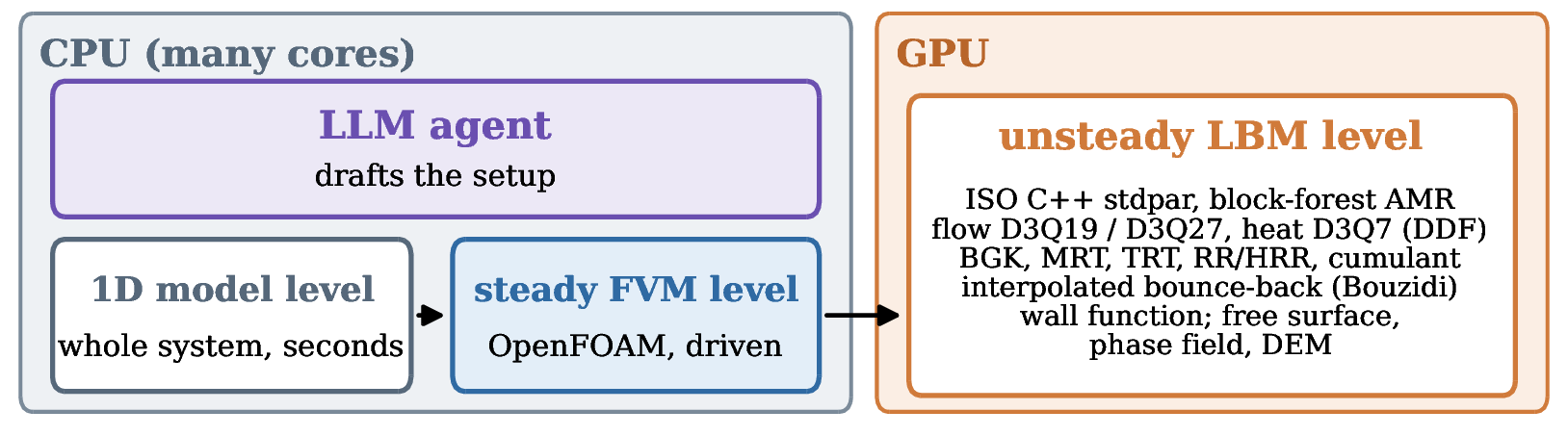
An open-source (Apache-2.0) environment where you work with an LLM agent and choose between a 1D model, steady FVM and unsteady LBM for each flow problem. The CPU runs the 1D model and steady FVM; the GPU runs unsteady LBM. The LLM only chooses the model and fills in parameters; the part that computes is deterministic C++ (source: gitlab.com/masaz/openrheo).
Showcase
Animations play inline (more in Showcase).
GPU liquid cold-plate multi-objective optimization (1D → Grace CPU FVM → Hopper H100 LBM in parallel)
| Unsteady thermal LBM (vortex shedding and temperature field in a Pareto-optimal pin-fin channel, 3.07 M cells) | 1D → FVM Pareto front → LBM verification and Miyabi-G simultaneous utilization |
|---|---|
 |
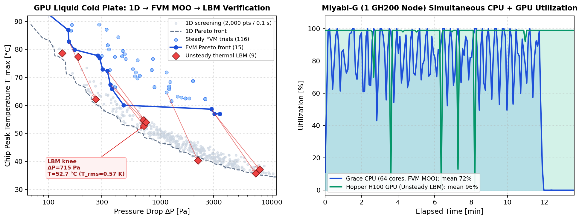 |
Three-level co-execution on a single Miyabi-G node (1 GH200, 13.7 min) for a 700 W-class staggered pin-fin cold plate. The 1D model screens 2,000 candidates in 0.1 s; Grace CPU (64 cores, 72% mean utilization) runs 116 steady FVM multi-objective evaluations (pressure drop ΔP vs. peak temperature T_max); simultaneously, Hopper H100 GPU (96% mean utilization, 3,933 MLUPS) verifies the emerging Pareto designs with 3.07 M-cell unsteady 3D thermal LBM, capturing Kármán vortex mixing and hotspot temperature fluctuations (T_rms = 0.57 K) missed by steady RANS → GPU cold-plate optimization
Automotive aero multi-objective optimization — Ahmed + diffuser (1D → Grace CPU FVM → Hopper H100 D3Q27 LBM in parallel)
| Unsteady aero D3Q27 Cumulant LBM (symmetry plane y = 0 velocity & \(C_p\), 5 mm, 13.8 M cells) | 1D → FVM → D3Q27 LBM Pareto verification (Ahmed 1984 exp. band) & Miyabi-G utilization |
|---|---|
 |
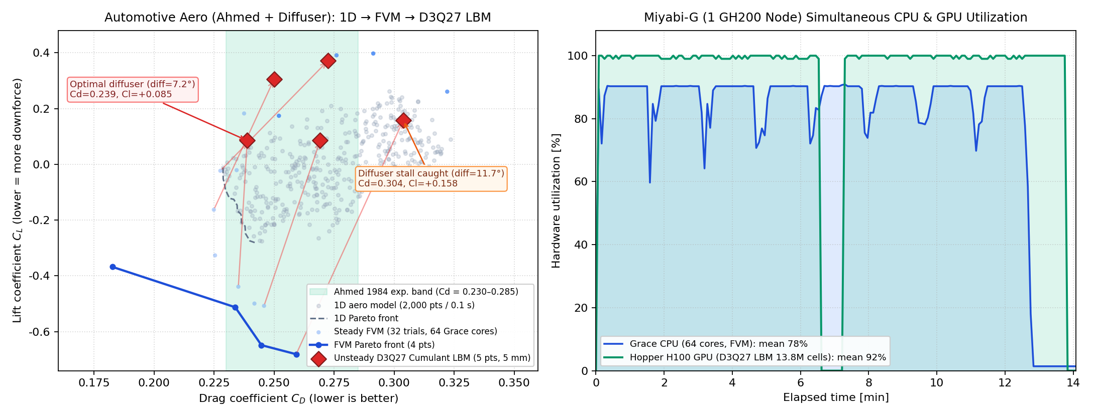 |
Three-parameter aerodynamic optimization (rear slant, underbody diffuser angle, ride height) on the canonical Ahmed body (ERCOFTAC Case 082, \(U_\infty = 40\text{ m/s},\; Re_H = 7.68\times 10^5\)) on Miyabi-G (1 GH200 node). The 1D aero model screens 2,000 configurations in 0.1 s; Grace CPU (64 cores, 78% mean / 91% peak utilization) runs 32 high-fidelity 440k-cell steady FVM (simpleFoam, 5 mm surface + 3 prism layers, \(C_D = 0.183\text{–}0.322\), baseline 25° \(C_D = 0.271\) vs. exp. \(0.285\)); simultaneously, Hopper H100 GPU (92% mean utilization, 331 MLUPS) verifies 5 Pareto vehicles using OpenRheo's production D3Q27 Cumulant + WALE + 4-level Octree AMR (5 mm finest, 13.8 M cells) + Bouzidi + Spalding + Kawai–Larsson friction solver. All three fidelities (1D, FVM, D3Q27 LBM) align inside the Ahmed 1984 experimental band (\(C_D = 0.230\text{–}0.285\)) (optimal 7.2° diffuser: FVM \(C_D = 0.235\) / LBM \(C_D = 0.239,\; C_L = +0.085\)), while unsteady LBM exposes 3D diffuser stall at 11.7° (\(C_D = 0.304\)) missed by steady FVM (baseline 25° validation: forest-ahmed-d3q27, \(C_{D,p} = 0.2278\) vs. exp. \(0.230\)).
Vehicle aerodynamics — DrivAer (unsteady LBM fed by a steady FVM solution)
| Unsteady LBM of the wake (velocity magnitude on the symmetry plane y = 0) | Steady FVM mean → LBM snapshot → wake time histories |
|---|---|
 |
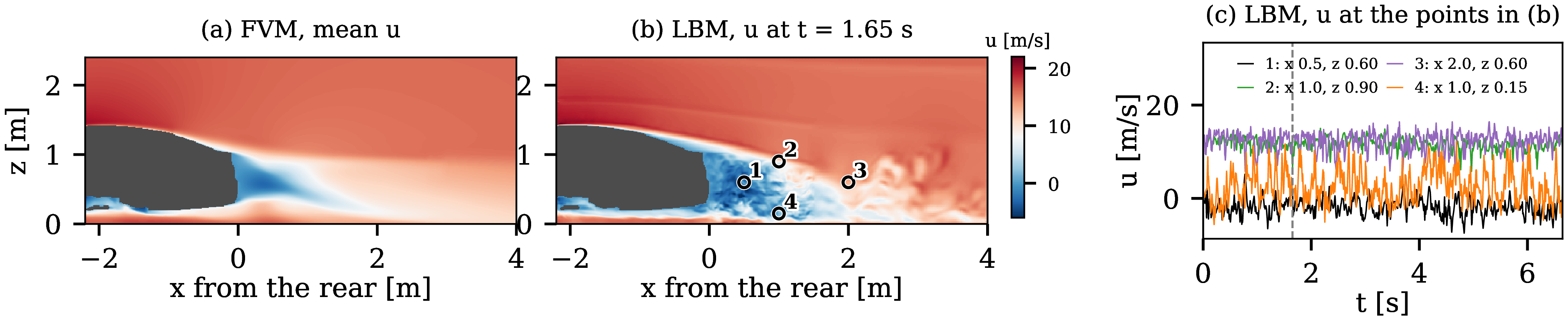 |
Steady FVM (3.43 M cells) gives Cd 0.257 (experiment 0.252). That velocity field becomes the inflow, and the wake is solved with LBM (19.82 M cells) in about 45 minutes on one GH200 of Miyabi-G → DrivAer fastback
Thermal environment of an apartment living room (unsteady LBM and steady FVM)
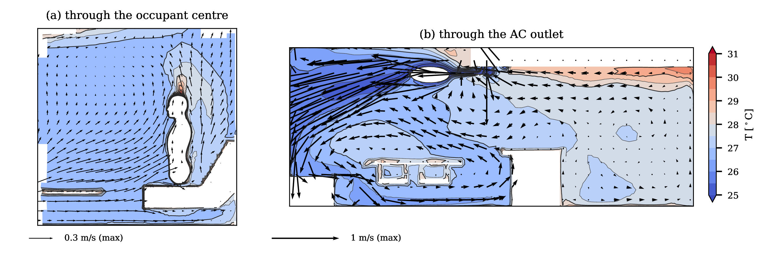
| Unsteady LBM (swinging circulator; wind speed on a vertical section through the seat) | Steady FVM temperature and wind speed (matches 56 measurements to RMS 0.63 K) |
|---|---|
 |
 |
Meshing and turbulence — rheoMesh and the wall-mounted cube
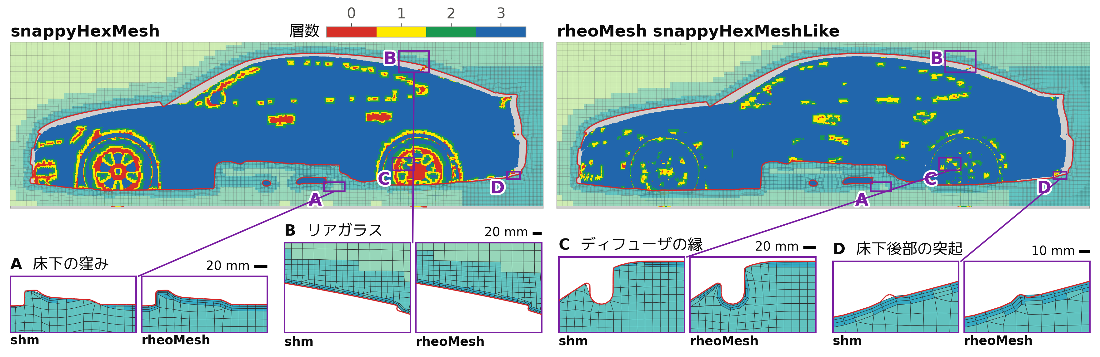
| rheoMesh layered mesh (DrivAer centre plane; left: snappyHexMesh, right: rheoMesh) | Vortices behind a wall-mounted cube (Q-criterion, ERCOFTAC case 41) |
|---|---|
 |
 |
Free surface, phase change and particles
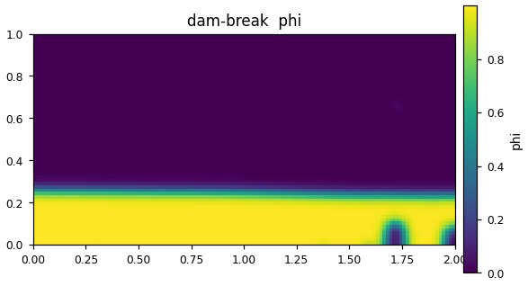
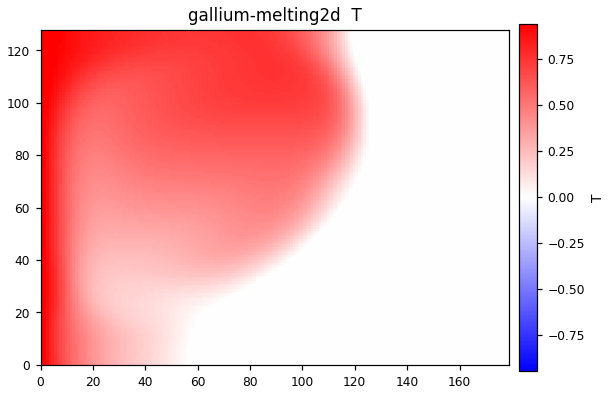
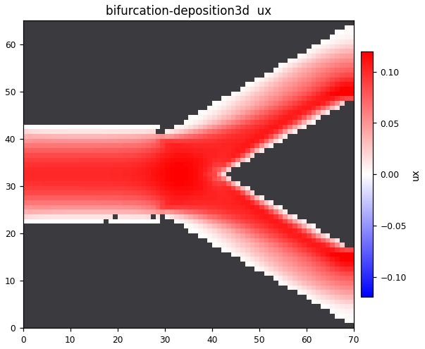
| Free surface: dam break | Heat and phase change: gallium melting | Particles and fluid: 3D bifurcation |
|---|---|---|
 |
 |
 |
Three levels
| Level | Role | Machine | What it is |
|---|---|---|---|
| 1D model | Solves the whole system in seconds. Go to FVM if you need distributions, to LBM if you need unsteadiness | CPU | Circuit models, coupling with a human thermoregulation model (JOS-3), etc. |
| Steady FVM | Finds spatial distributions | CPU (many cores) | Builds and runs tuned OpenFOAM cases |
| Unsteady LBM | Finds what only unsteady flow gives (fluctuations, spectra, draught sensation, ...) | GPU | A custom kernel in ISO C++ standard parallel algorithms (stdpar): block-forest AMR, D3Q19 / D3Q27, D3Q7 for heat, free surface, phase field, DEM |
Hand-over of fields between the levels is checked in the multi-fidelity (1D ⇄ FVM ⇄ LBM) cases. Each physics module is guarded by ctests against the values of the original papers (Architecture).
The mesher: rheoMesh
- Reads the snappyHexMeshDict as is, builds layered FVM meshes with threads, and also writes the LBM block forest from the same octree.
- 83 / 88
Mesh OKon all 88 OpenFOAM tutorials (83 / 83 runnable = 100 %, OpenFOAM-13: 23 / 23). On the course DrivAer (3 layers), 27.3 s versus 37.4 s for snappyHexMesh (skewness > 3 faces: 172 → 27). - → rheoMesh (design, comparisons, how to run)
Validation status
The 81 cases are listed by field under "Categories" below. Many are still a single-point comparison at a single grid resolution. Cases that show the grid-convergence order (T0), cases with an automatic gate (T1), one-off comparisons (T2) and demos (T3) are distinguished in Validation status; unmeasured columns are shown as "not measured".
Highlights and changelog
- 2026-11-21 rheoMesh: 82/88
Mesh OKon all 88 tutorials (OpenFOAM-13: 23/23), MPI bit-identity 37/37, layered 22.6 M-cell DrivAer mesh. - 2026-11-20 OpenCAE Symposium 2026 talk: figures and key numbers of the talk, section by section.
- 2026-10-13 Wiki published (DrivAer, wall-mounted cube and more).
Detailed history is in the rheoMesh development log; all pages are in the page index. See also Validation status · Known issues. To run it: GitLab README.
Categories
Single-phase basics, turbulence and external flow
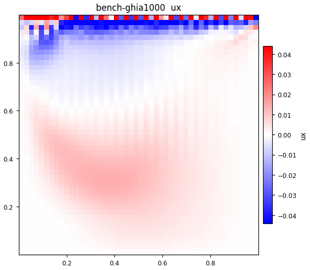 Laminar flow and analytic verification (17) Laminar cases that can be checked directly against analytic solutions and classic benchmarks. They pin down the foundation of the solver. T0 3 / T1 3 / T2 10 / T3 1 |
 Turbulence (checked against DNS/LES) (9) Turbulent cases checked against DNS or experiment. Judged by statistics such as decay rates and the log law. T0 1 / T1 0 / T2 8 / T3 0 |
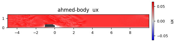 External flow and wind engineering (11) Separated flows around vehicles and buildings. Assessed by drag coefficients and wind-speed profiles. T0 0 / T1 0 / T2 9 / T3 2 |
Free surface, multiphase, heat, scalar transport and coupling
Free surface (11) Dam breaks and wave loads with single-phase free-surface LBM (VOF). Compared with experimental values as time series. T0 0 / T1 0 / T2 9 / T3 2 |
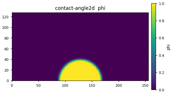 Two-phase flow (phase field) (6) Bubbles, surface tension and wetting. High-density-ratio Allen-Cahn phase field. T0 0 / T1 1 / T2 5 / T3 0 |
Heat transfer and phase change (4) Boussinesq natural convection and melting. Double-distribution-function (DDF) thermal LBM. T0 0 / T1 4 / T2 0 / T3 0 |
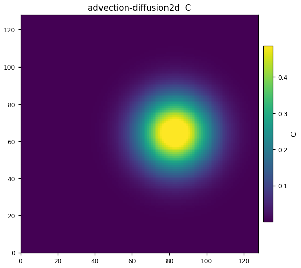 Advection-diffusion, reaction and radiation (4) Passive scalar transport and radiative heat transfer. Can be verified against analytic solutions down to the order of convergence. T0 1 / T1 2 / T2 1 / T3 0 |
 Electrochemistry and microflows (2) Electric double layers and electro-osmotic flow. Up to Poisson-Nernst-Planck. T0 0 / T1 1 / T2 1 / T3 0 |
Particles and fluid-structure interaction (7) Two-way coupling through moving boundaries and momentum exchange. Settling, DKT, valves. T0 0 / T1 0 / T2 7 / T3 0 |
Numerical verification, multi-fidelity and optimization
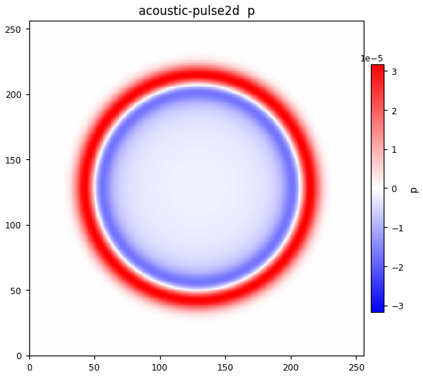 AMR and numerical verification (3) Verification of the numerical schemes themselves, such as spurious noise at coarse-fine interfaces and the speed of sound. T0 1 / T1 0 / T2 2 / T3 0 |
Multi-fidelity (1D ⇄ FVM ⇄ LBM) (4) The same circuit is solved with handbook correlations, RANS and LBM, and the disagreement between them is measured. The subject is the hand-off of resolved coefficients back to 1D, and its conventions. T0 0 / T1 4 / T2 0 / T3 0 |
Optimization, inverse problems and uncertainty (3) Adjoint gradients, parameter identification and uncertainty propagation. Verified where the true value is known. T0 3 / T1 0 / T2 0 / T3 0 |
About the name: "Rheo" comes from the Ancient Greek verb ῥέω (rheō, "to flow").