stefan-melting2d
English | Japanese
« Home · « Heat transfer and phase change
Enthalpy-method thermal LBM -- one-phase Stefan melting problem. A semi- infinite solid initially at the melt temperature T_m suddenly has its x=0 face raised to T_wall > T_m; the solid-liquid front x_f(t) advances into the domain following the classical Stefan similarity solution. This is a pure- conduction test (no flow, u = 0), so only the scalar (thermal) population is evolved -- the D2Q5 advection-diffusion LBM of thermal_cavity2d.cpp with the advection velocity set to zero, plus a latent-heat source. C++20 stdpar.
Geometry

Animation
Fields
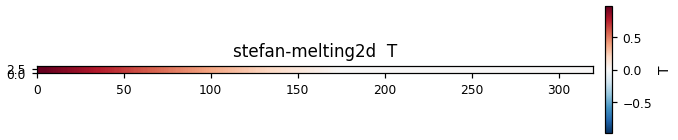
The fields this computation wrote at its last output step, plotted as they are. 3D cases show the mid-plane.
Results
Enthalpy-method verification of one-phase Stefan melting — pure conduction with no flow (u = 0) + latent heat, following the moving solid–liquid front on a fixed grid. Nx = 320 (Ny = 4, periodic in y, so effectively 1D), 120000 steps, St = 1.000, α = 1/6 (τ_g = 3α + 1/2 = 1.0000), L = 1.0000, cp = 1.000. Wall-clock 1.42 seconds.
- Front position: against the similarity solution x_f(t) = 2λ√(αt), the comparison in the log every 10000 steps is within 0.1% on every row. Example: at step 10000, 50.697 vs analytical 50.628; at step 120000, 175.297 vs 175.380. Check of the analytical value: 2 × 0.620063 × √(0.16667 × 120000) = 1.240126 × √20000 = 175.38 ✓.
- Similarity coefficient: from the x_f–√t fit, λ_meas = 0.620052 vs exact λ_exact = 0.620063, error −0.0018% (lambda_err_pct in the RESULT line). The exact value is the root of a transcendental equation; check: 0.620063 × e^{0.384478} × erf(0.620063) = 0.5642 = 1/√π ✓.
- Temperature field: relative L2 against the error-function profile in the liquid region (n = 175 cells) = 2.4253e-04. Not only the front position but the whole field agrees.
Recovering λ to 5 digits without tracking the front explicitly — this is as sharp a gate as one could ask for
in verifying the enthalpy closures
(enthalpy_liquid_fraction / latent_heat_source, closures.hpp), and
gallium-melting2d, which adds convection, uses these components as they are.
Governing equations
The x = 0 face of a semi-infinite solid (initial temperature = melting point T_m) is raised to T_wall at t = 0. Classical Stefan similarity solution (Carslaw–Jaeger / Alexiades–Solomon):
\[
x_f(t)=2\lambda\sqrt{\alpha t},\qquad
\lambda e^{\lambda^2}\mathrm{erf}(\lambda)=\frac{St}{\sqrt{\pi}},\qquad
St=\frac{c_p(T_{\rm wall}-T_m)}{L}
\]
\[
T(x,t)=T_{\rm wall}\Big(1-\frac{\mathrm{erf}(x/2\sqrt{\alpha t})}{\mathrm{erf}\lambda}\Big)
\]
On the LBM side, the enthalpy method (Jiaung–Ho–Kuo 2001): total enthalpy H = c_p T + L·f_l (f_l ∈ [0,1] is the liquid fraction). A D2Q5 scalar LBM carries the sensible heat T = Σ g_i, and the latent heat enters as a source S = −(L/c_p) df_l/dt inside the collision. f_l is inverted from the local enthalpy every step (isothermal phase change pinned at T_m), and the front emerges from the grid as the 0–1 transition of f_l — no front tracking and no remeshing needed. Since u = 0, the D2Q5 of thermal_cavity2d is used as a pure diffusion operator, with α = c_s²(τ_g − 1/2). The boundaries are anti-bounce-back Dirichlet with T_wall at x = 0 and T_m at x = L (the right end is placed far beyond the front to mimic a semi-infinite domain); y is periodic.
Code walkthrough
Source (281 lines) and closures.hpp.
%%{init: {'themeVariables': {'fontSize': '11px'}}}%%
flowchart LR
    W["x=0: T_wall<br/>anti-BB Dirichlet"] --> LQ["Liquid f_l=1<br/>error-function profile"]
    LQ --> F(("Front x_f(t)<br/>0<f_l<1")) --> S["Solid f_l=0, T=T_m"]
S --> E["x=L: T_m Dirichlet<br/>(stand-in for semi-infinite)"]- λ root-finding — Solve the monotonic transcendental equation by bisection to get lambda_exact.
- collide — D2Q5 BGK + latent-heat source.
enthalpy_liquid_fractionupdates f_l, andlatent_heat_sourceturns df_l/dt into the source. - stream + BC — Periodic y, anti-BB at both x ends.
- Diagnostics — Every 10000 steps, front position at f_l = 1/2 vs the analytical value. At the end, the λ fit, the liquid-region temperature L2, the RESULT line, and front/profile CSVs.
Build & run
cmake -S native -B native/build && cmake --build native/build -j
./native/build/orheo-stefan-melting2d
stefan_melting2d [Nx] [steps] [St] [alpha] [out_prefix] [Ny]
Cost of the computation that made the figures on this page (Miyabi-G Grace CPU (72 cores, -stdpar=multicore)): 1.4 s wall.
Things to try
- St sweep:
stefan_melting2d 320 120000 0.1— the smaller St, the slower the front (λ(0.1) ≈ 0.22), and the better the quasi-steady approximation. Is the accuracy of λ_meas maintained? - Change τ_g: shifting α away from 1/6 so that τ_g ≠ 1 changes the error balance between the anti-BB Dirichlet and the latent-heat source. How far does −0.0018% move?
- Bring the right end closer: with Nx = 200, observe the time at which the front "feels" the Dirichlet T_m of the right wall — a hands-on lesson in how the semi-infinite approximation breaks down.
- On to gallium-melting2d: adding Carman–Kozeny drag and buoyancy to the same 2 closures gives melting with convection. Read and compare the differences.
Validation
| Tier | T1 — automatic gate |
| QoI | front_position |
| Reference | analytic one-phase Stefan similarity solution |
| Gate | 🧩 module gate (closures) |
Source & run details
| Item | Value |
|---|---|
| Target | orheo-stefan-melting2d |
| Source | native/benchmarks/stefan_melting2d.cpp |
| Lattice | D2Q9 |
| GPU twin | no |
| Modules | closures.hpp |
| Gallery run | 2026-07-27 @ 7628c0cf |
| Args | `` |
| Wall time | 1.42 s |
| CPU time | 94.81 s |
| Device | Miyabi-G Grace CPU (72 cores, -stdpar=multicore) |
Computation log
The actual output of this computation (head and tail).
stefan_melting2d Nx=320 Ny=4 steps=120000 St=1.000 alpha=0.16667 tau_g=1.0000 L=1.0000 cp=1.000  lambda_exact=0.620063
  step 10000: x_f=50.697  (analytic 50.628)
  step 20000: x_f=71.657  (analytic 71.599)
  step 30000: x_f=87.775  (analytic 87.690)
  step 40000: x_f=101.162  (analytic 101.256)
  step 50000: x_f=113.124  (analytic 113.207)
  step 60000: x_f=124.009  (analytic 124.013)
  step 70000: x_f=133.981  (analytic 133.949)
  step 80000: x_f=143.117  (analytic 143.197)
  step 90000: x_f=151.940  (analytic 151.884)
  step 100000: x_f=160.053  (analytic 160.099)
  step 110000: x_f=167.959  (analytic 167.914)
  step 120000: x_f=175.297  (analytic 175.380)
x_f(final)=175.297  lambda_meas=0.620052  lambda_exact=0.620063  err=-0.00%
References
- W.-S. Jiaung, J.-R. Ho & C.-N. Kuo, Numerical Heat Transfer B 39 (2001) 167–187 — enthalpy-method LBM.
- X. He, S. Chen & G. D. Doolen, J. Comput. Phys. 146 (1998) 282.
- H. S. Carslaw & J. C. Jaeger, Conduction of Heat in Solids, 2nd ed., Oxford (1959), Ch. XI.
- V. Alexiades & A. D. Solomon, Mathematical Modeling of Melting and Freezing Processes, Hemisphere (1993), Ch. 1–2.