One-dimensional gallery
English | 日本語
In development
The components on this page are in development branches and not yet in the public source (as of 2026-11-20). The figures were made with the C++ code of those branches.
This page shows the results of the Modelica Standard Library (MSL 4.1.0) port as figures. In every figure the solid colour line is OpenRheo and the black dashed line is the reference. Unless stated otherwise, the reference is OpenModelica 1.27.1. Deviation panels use a log scale; points where the deviation is exactly 0 are drawn at the bottom edge. The text and tables are on One-dimensional models. The scripts that make the figures are in tools/onedim_gallery/ of the site repository.
Shared DAE core
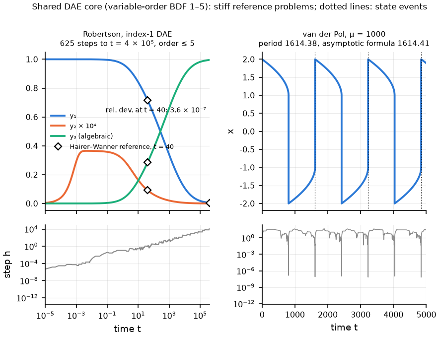
Two stiff reference problems. The Robertson kinetics match the Hairer–Wanner reference at t = 40 to 3.6 × 10⁻⁷ (relative). The van der Pol period (μ = 1000) is 1614.38, 1.9 × 10⁻⁵ from the asymptotic formula (1614.41).
Media
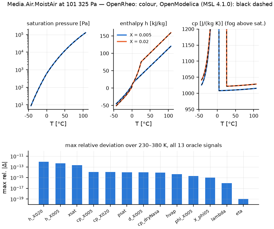
Thirteen moist-air quantities over 230 to 380 K. The largest relative deviation is 9.7 × 10⁻¹³ (enthalpy at X = 0.02).
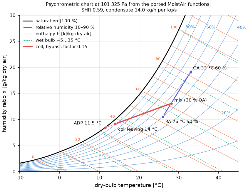
Every line of the chart is computed with the ported MoistAir functions. After mixing with 30 % outdoor air, the coil cools the air to 14 °C. The ADP is 11.5 °C and the sensible heat ratio 0.59. The bypass factor recomputed from the leaving state is 0.15, as set.
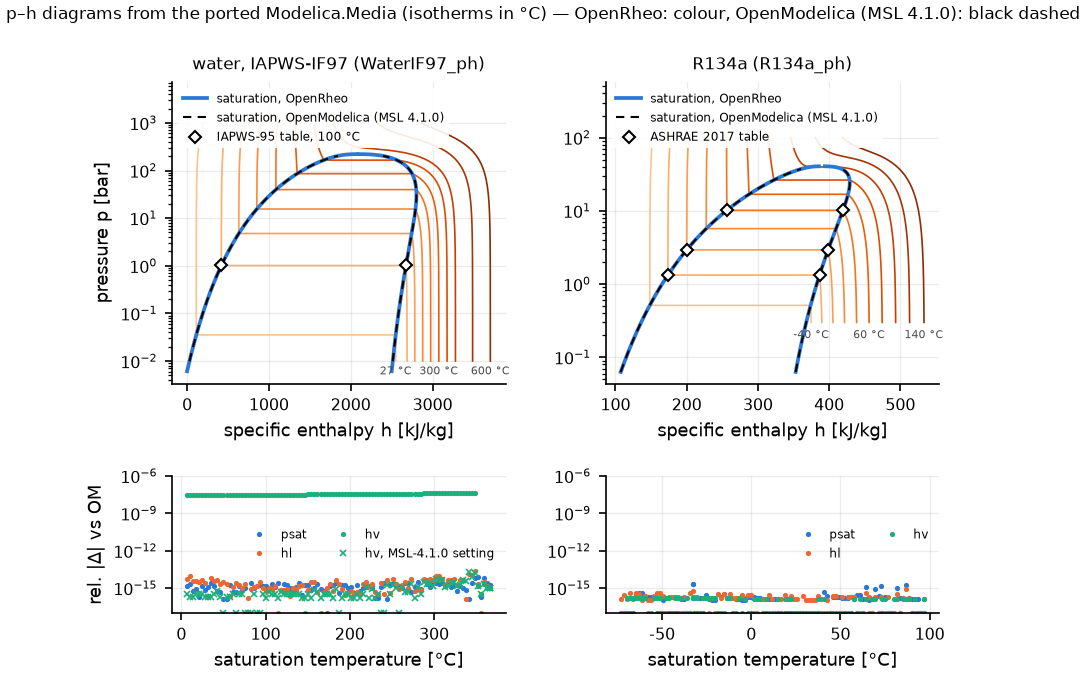
p–h diagrams from the ported IF97 and R134a media. The saturation lines match OpenModelica to 2 × 10⁻¹⁴ relative or better. The exception is the saturated-vapour enthalpy of water: 4.6 × 10⁻⁸ with the default (IAPWS-correct) setting and 2 × 10⁻¹⁴ with the MSL-4.1.0 setting. The diamonds are IAPWS-95 and ASHRAE table values.
Control blocks and tables
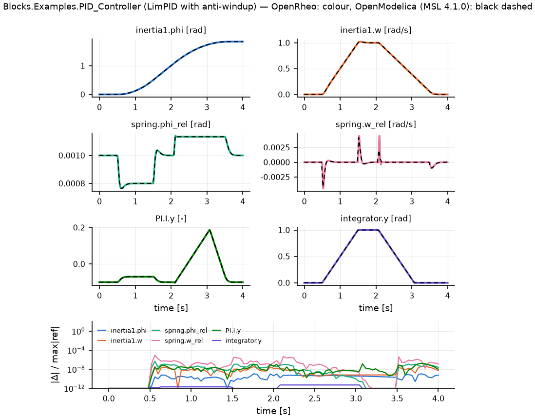
The six states of Blocks.Examples.PID_Controller. The LimPID saturates and its anti-windup acts. The deviation is at most 8.7 × 10⁻⁶ of each state's largest value (spring.w_rel).
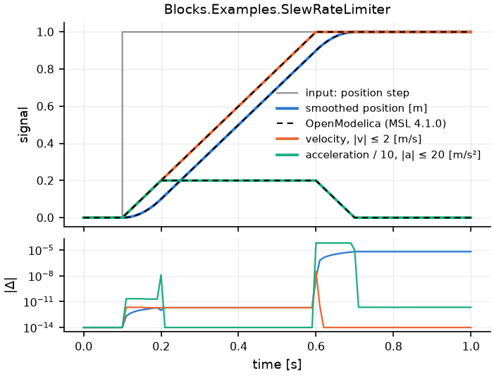
A position command with limited velocity and acceleration. The largest deviation is 6.6 × 10⁻⁵ in the acceleration (limit 20).
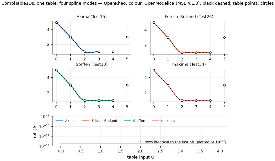
One table interpolated with Akima, Fritsch–Butland, Steffen and makima. The values match OpenModelica to the last bit.
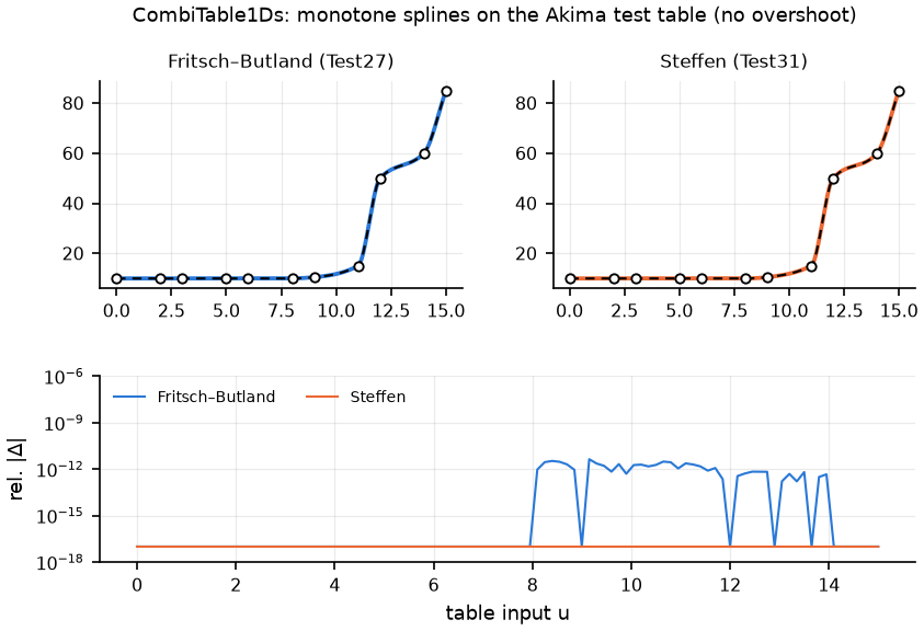
The monotone splines do not overshoot on flat parts. The largest relative deviation is 4.3 × 10⁻¹².
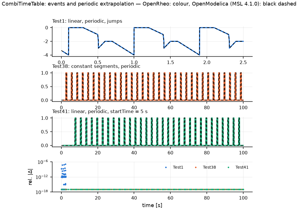
Jumps, constant segments, periodic extrapolation and a start-time shift. The largest relative deviation is 1.2 × 10⁻⁷; it comes from the time stamp OpenModelica writes for the row right after an event.
Heat transfer
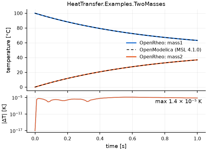
Two heat capacitors joined by one conductor. The deviation from OpenModelica is 1.4 × 10⁻⁵ K. This is the error of the OpenModelica result itself: OpenRheo matches the analytic solution to 6.7 × 10⁻⁹ K.
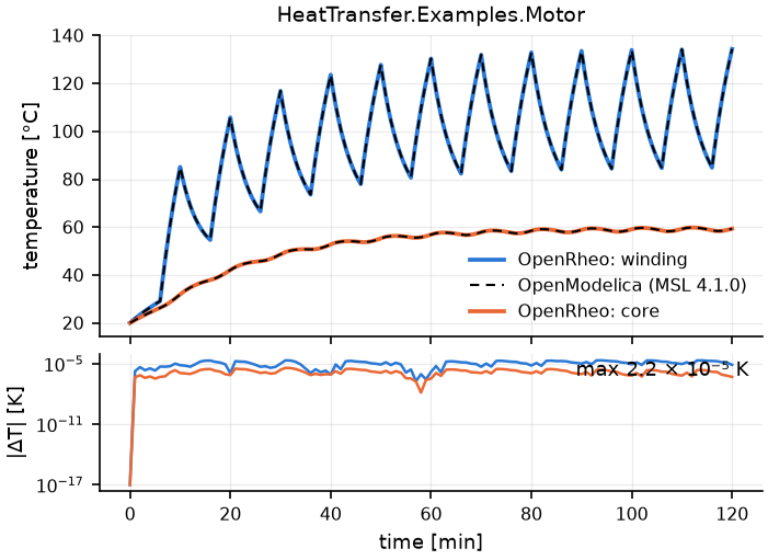
Winding and core of a motor heated by periodic losses. The largest deviation is 2.2 × 10⁻⁵ K (winding).
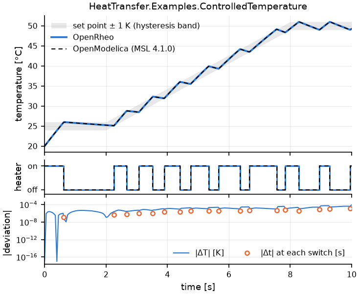
A heater under on/off control. All 18 switches match; the largest time difference is 1.4 × 10⁻⁵ s and the largest temperature difference 8.4 × 10⁻⁵ K.
Multilayer wall
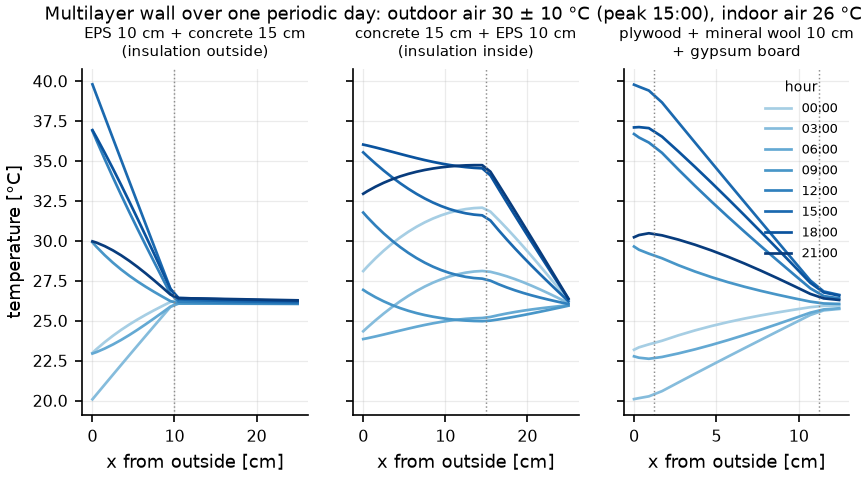
One periodic day with outdoor air at 30 ± 10 °C (peak at 15:00) and indoor air at 26 °C. Profiles every three hours; the dotted lines are layer boundaries.
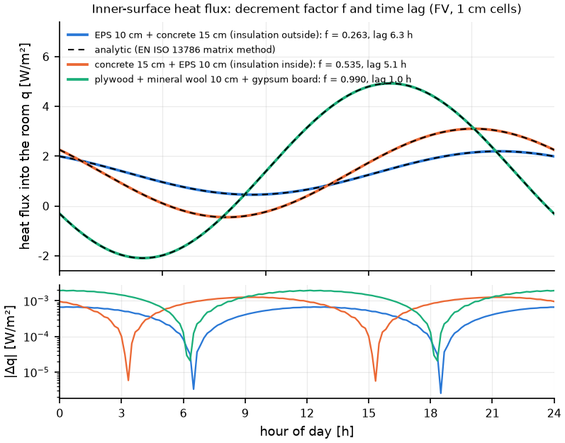
The heat flux into the room against the analytic solution of the EN ISO 13786 matrix method. The decrement factors differ by 0.07 % or less, the time lags by 7 s or less, and the heat flux by at most 2 × 10⁻³ W/m².
Room heat balance (demonstration)
A demonstration
This room uses typical constructions and loads and synthetic weather. It is not compared with measurements.
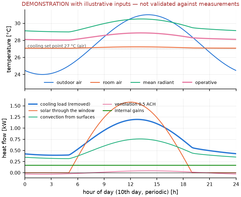
The tenth day of one apartment room (south window, 0.5 air changes per hour, cooling set point 27 °C). The peak cooling load is 1.19 kW (about 12:50), the daily cooling 17.3 kWh. The operative temperature stays between 28.0 and 28.9 °C.
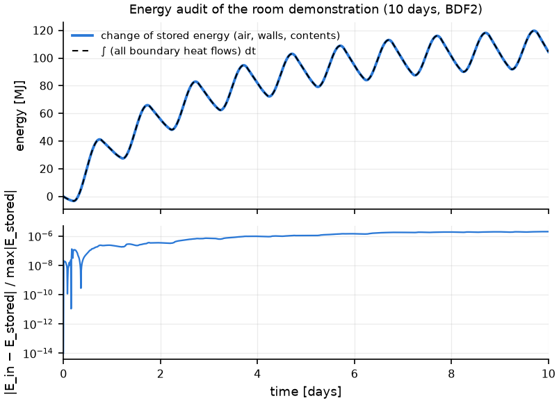
The integral of all boundary heat flows against the change of stored energy. Over 10 days they differ by at most 2 × 10⁻⁶ of the largest stored energy.
FluidHeatFlow and FluxTubes
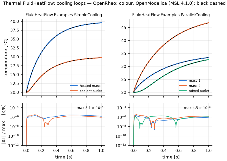
Two cooling examples of Thermal.FluidHeatFlow. The temperature deviation is at most 4.5 × 10⁻⁶ of the largest temperature (in K).
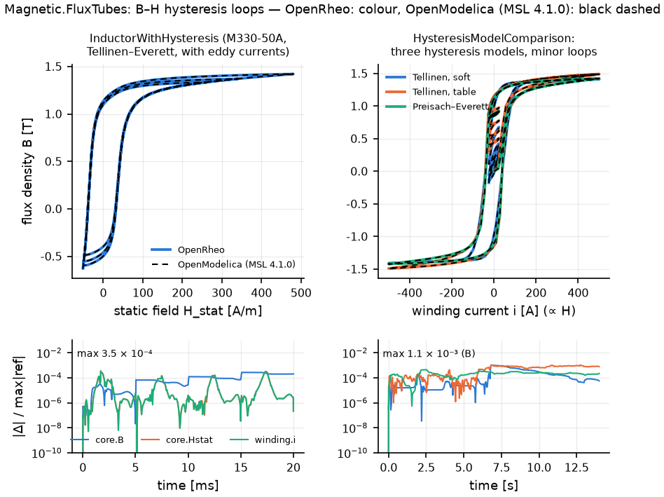
B–H hysteresis loops of Magnetic.FluxTubes: left, an inductor with eddy currents; right, minor loops of three hysteresis models. The largest deviations are 3.5 × 10⁻⁴ and 1.1 × 10⁻³ (B, relative to its largest value).
Fluid networks
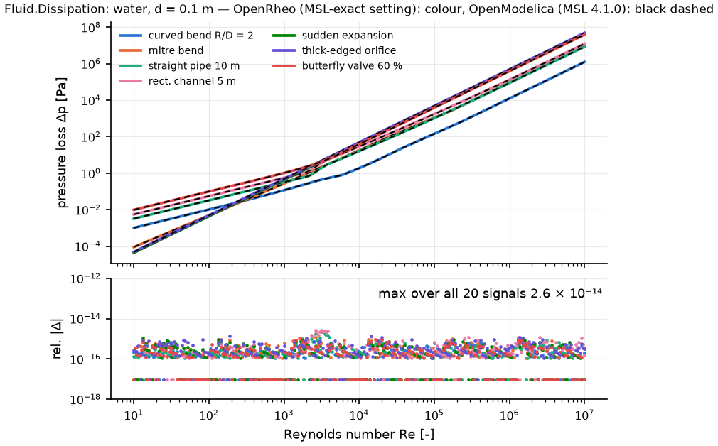
The pressure-loss functions with the MSL-exact setting over Re = 10 to 10⁷. Over all 20 signals the largest relative deviation is 2.6 × 10⁻¹⁴.
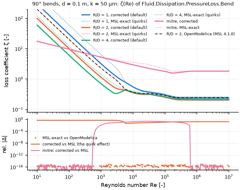
Bend loss coefficients. The MSL-exact setting matches OpenModelica to 1 × 10⁻¹⁵. The corrected default is half of MSL's value in laminar flow and, at high Re, 17 % lower for the curved bend and 18 % lower for the mitre bend (findings).
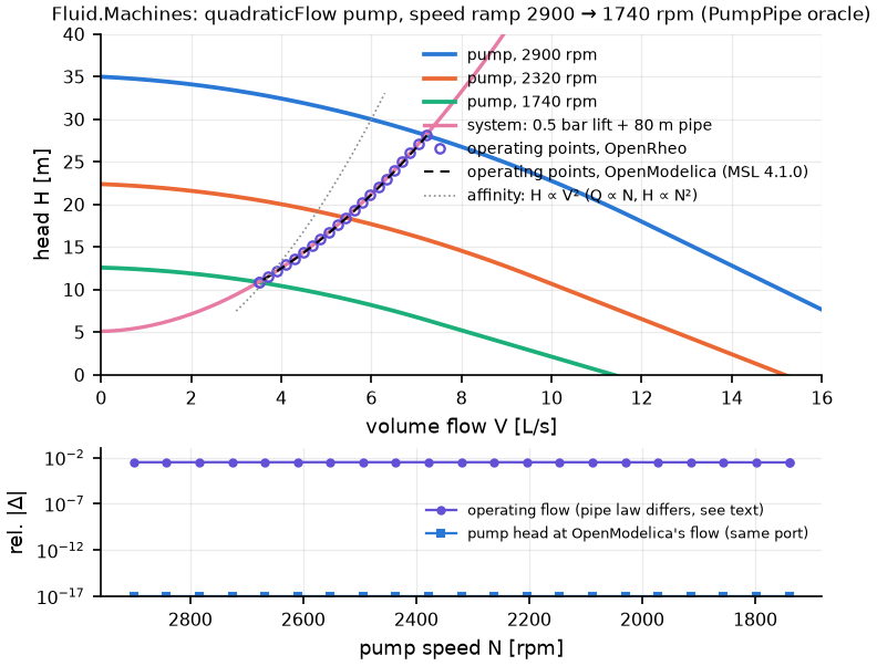
Operating points while the speed drops from 2900 to 1740 rpm. The pump head matches OpenModelica exactly. The flow differs by 0.31 % because the pipe laws differ (MSL WallFriction.Detailed, OpenRheo Dissipation.StraightPipe).
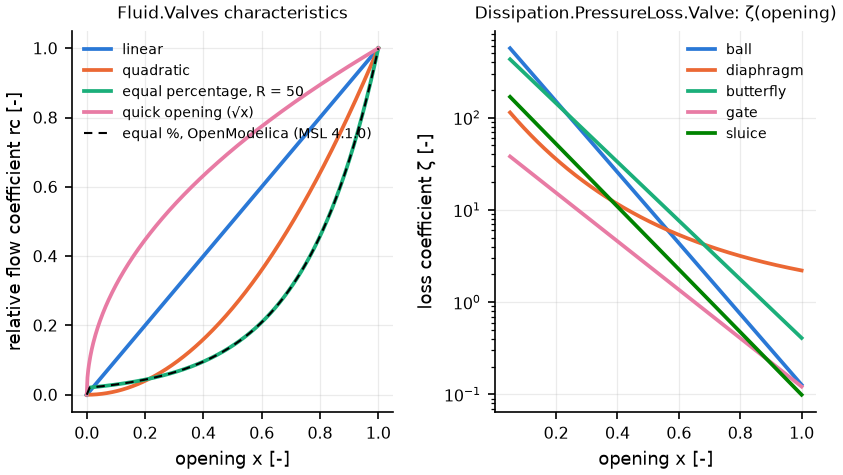
Inherent valve characteristics and the loss coefficient of each valve geometry. The equal-percentage characteristic matches OpenModelica to 8 × 10⁻¹⁶.
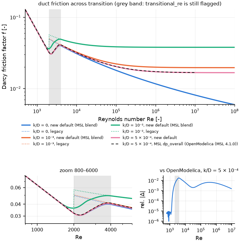
The new duct default (MSL's smooth transition) and the old law, which jumped by 54 % at Re = 2000. Above Re = 4000 the default is still Colebrook, up to 1.7 % from MSL's formula.
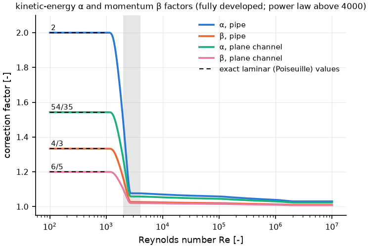
Kinetic-energy and momentum correction factors: exact values for laminar flow (pipe 2 and 4/3, plane channel 54/35 and 6/5) and power-law integrals for turbulent flow. In a pipe at Re = 10⁵, α = 1.059.
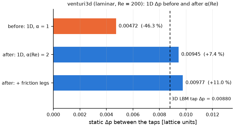
The 1D Δp of a laminar venturi (Re = 200) against the 3D LBM value. With α = 1 the 1D value is 46 % low; with α(Re) = 2 it is 7.4 % high. The numbers in this figure are copied from the design record.
Multibody systems
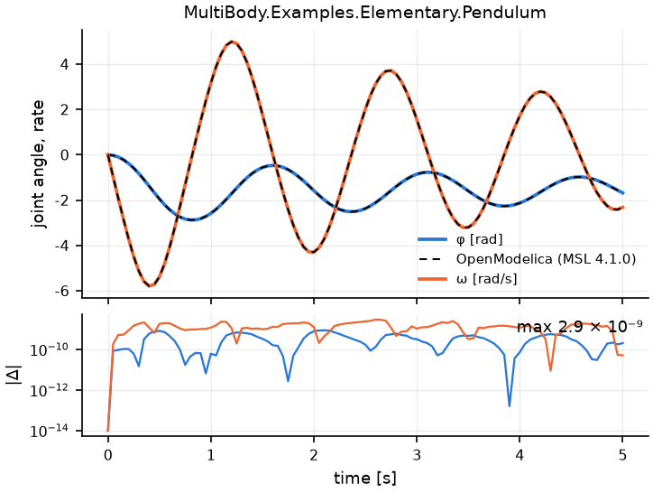
A damped pendulum. The largest deviation is 2.9 × 10⁻⁹.
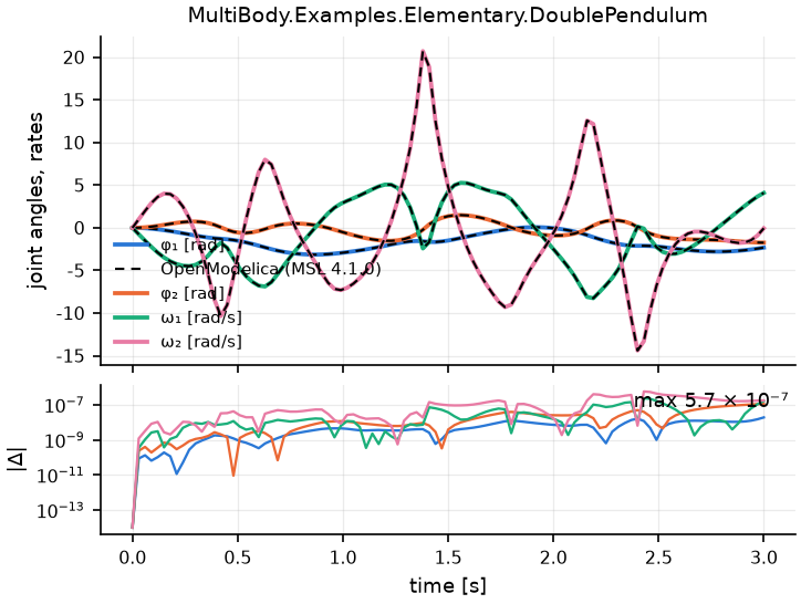
A double pendulum. The largest deviation is 5.7 × 10⁻⁷ rad/s.
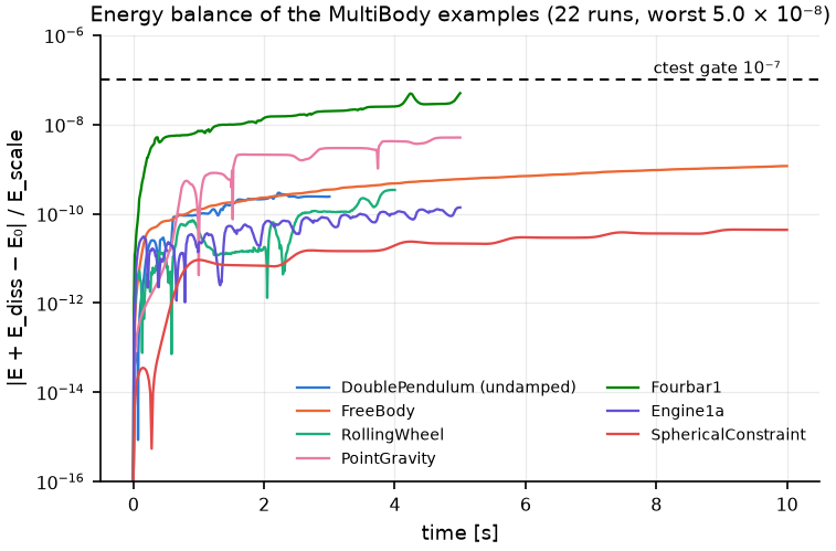
The change of total energy plus dissipated energy. Over 22 runs the largest value is 5 × 10⁻⁸ (relative).
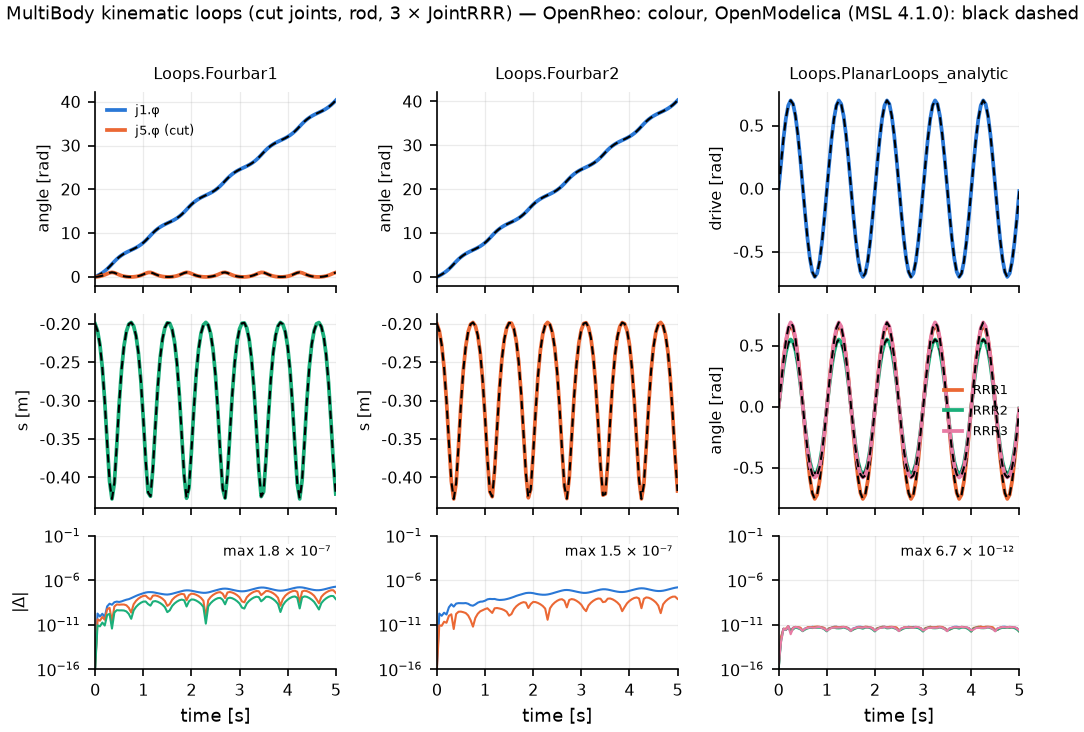
Loops closed by a cut joint, a rod and JointRRR assemblies. The largest deviation is 1.8 × 10⁻⁷ (Fourbar1).
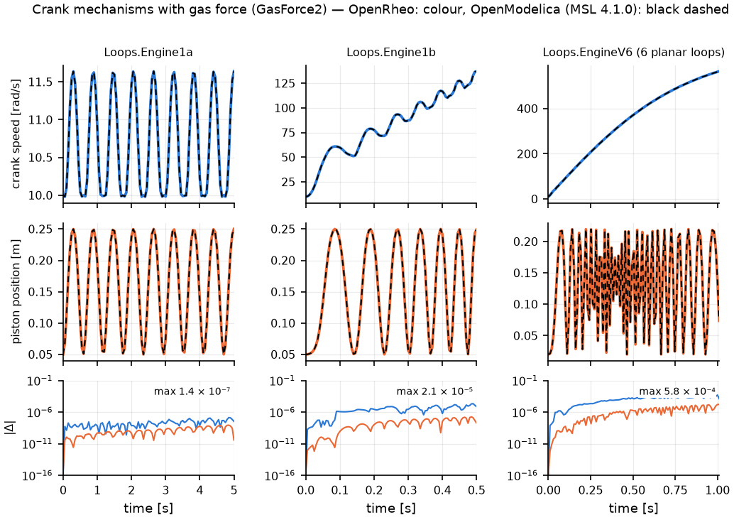
Crank mechanisms driven by gas force. The OpenModelica reference has no gas pressure, so the figure shows crank speed and piston position. The largest deviations are 1.4 × 10⁻⁷ (Engine1a), 2.1 × 10⁻⁵ (Engine1b) and 5.8 × 10⁻⁴ (EngineV6, at a crank speed of 565 rad/s).
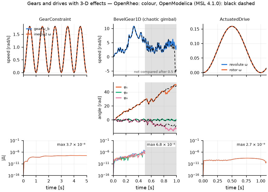
GearConstraint, BevelGear1D and ActuatedDrive. BevelGear1D is chaotic and compared only for t ≤ 0.5 s (the grey part is not compared). The largest deviation is 6.8 × 10⁻⁶.
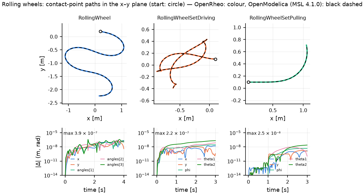
Contact-point paths of rolling wheels. The largest deviation is 3.9 × 10⁻⁷.
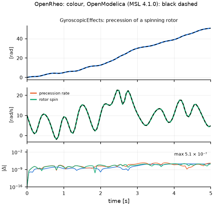
Precession of a spinning rotor. The largest deviation is 5.1 × 10⁻⁷.
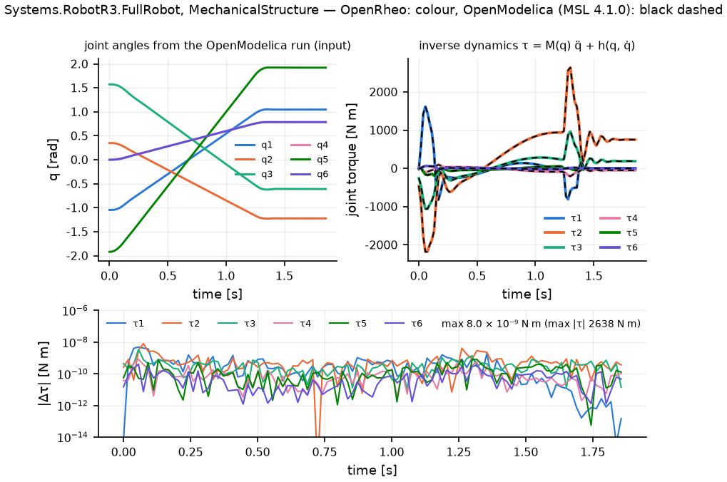
The mechanical structure of RobotR3. From the joint angles, rates and accelerations of the OpenModelica run, OpenRheo's equations of motion give the joint torques. They differ by at most 8 × 10⁻⁹ N m; the largest torque is 2638 N m.
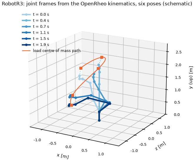
A schematic of the same run: the joint positions at six instants.
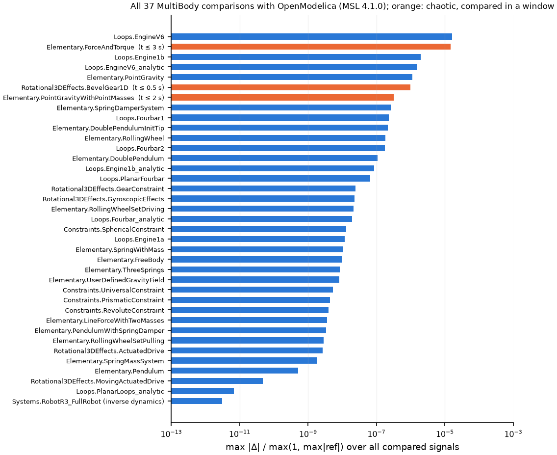
The largest deviation of all 37 comparisons. Orange marks the chaotic examples, compared only up to t = 3 s (ForceAndTorque), 2 s (PointGravityWithPointMasses) and 0.5 s (BevelGear1D). After that, even the OpenModelica result depends on the solver tolerance.
1D mechanics (Translational, Rotational)
As in the ctest, the deviation is relative to the value range of the reference.
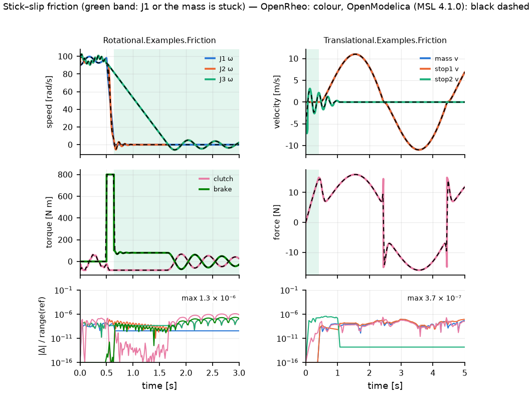
Stick-slip friction; the green band marks the stuck time. The largest deviations are 1.3 × 10⁻⁶ and 3.7 × 10⁻⁷.
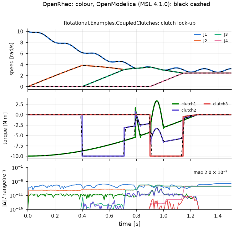
Three clutches lock up in turn. The largest deviation is 2 × 10⁻⁷.
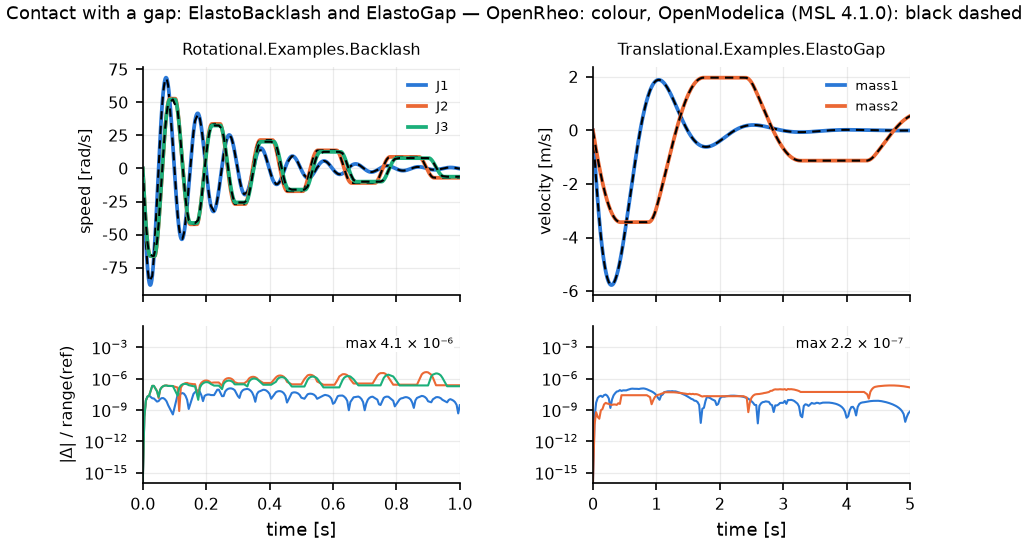
ElastoBacklash and ElastoGap. The largest deviations are 4.1 × 10⁻⁶ and 2.2 × 10⁻⁷.
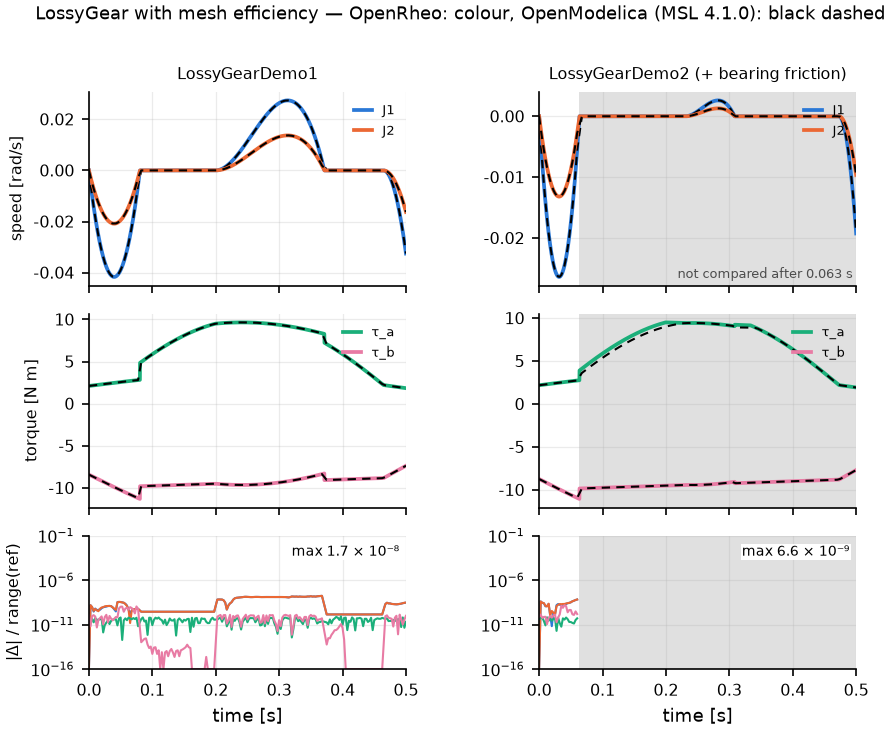
A gear with mesh efficiency. Demo2 is compared only for t ≤ 0.063 s. After that the gear and the bearing friction are both stuck, and the split of the two sticking torques is not unique; OpenModelica's split comes from its linear solver. The largest deviations are 1.7 × 10⁻⁸ and 6.6 × 10⁻⁹.
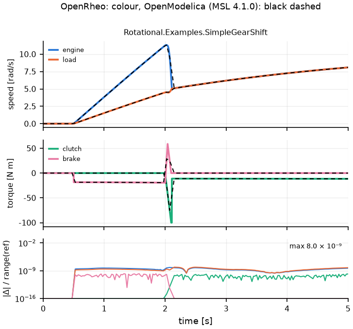
A gear shift with a clutch and a brake. The largest deviation is 8 × 10⁻⁹.
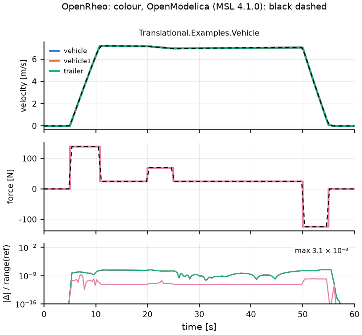
The vehicle and trailer example. The largest deviation is 3.1 × 10⁻⁸.
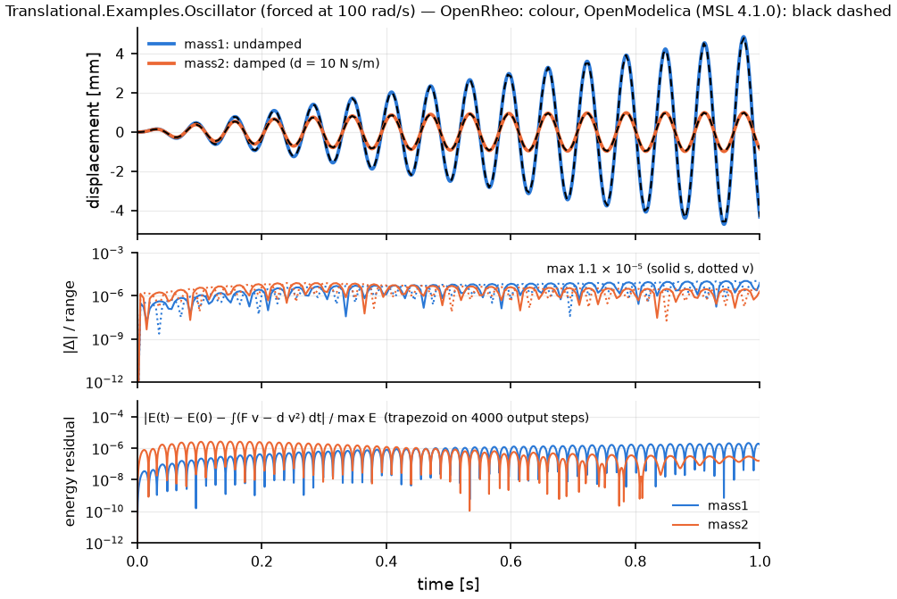
Two forced oscillators, undamped and damped. The largest deviation is 1.1 × 10⁻⁵. The energy-balance residual is 2.6 × 10⁻⁶ or less, the size of the trapezoid-rule error on 4000 output steps.
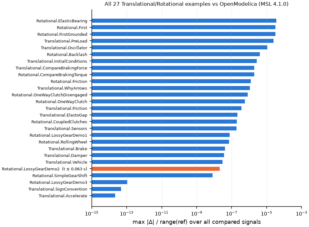
The largest deviation of all 27 examples. The worst is 3.6 × 10⁻⁵ (ElasticBearing).