Multi-fidelity: 1D, steady FVM and LBM
English | Japanese
OpenRheo answers each question with the cheapest tier that can answer it: a 1D network model, a steady RANS solve in OpenFOAM, or the unsteady AMR-LBM. A fixed rule, not the LLM, decides when a question moves up; the local LLM drafts the setup and fills a bounded set of keys. This page shows the tiers and the rule, what the 1D library holds, the cases that were taken up the ladder, and what is open. Several cases have their own pages, linked below.
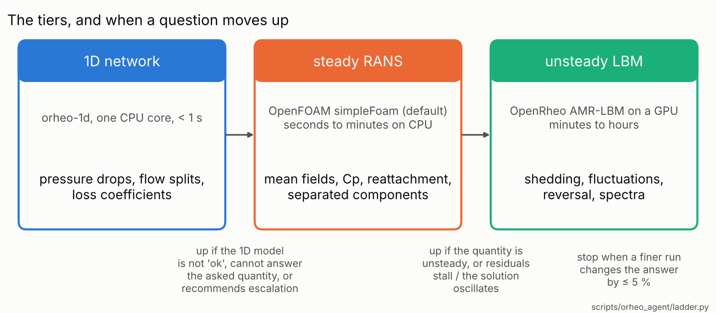
The rule
The rule is in scripts/orheo_agent/ladder.py:
- 1D is enough when its summary says
ok, none of the asked quantities is on itscannot_answerlist, and it does not recommend escalation. - Steady RANS is skipped when every asked quantity is unsteady (a spectrum, a fluctuation); a mix of steady and unsteady quantities runs RANS and then LBM. RANS is enough when the residuals reach their thresholds and the quantity has reached a plateau. A stall (residuals not falling) or an oscillation (six or more zero crossings) sends the question up.
- LBM runs at increasing resolution and stops when the answer changes by 5 % or less.
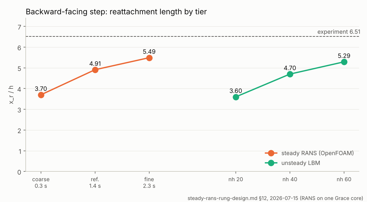
The steady tier runs OpenFOAM by default. An in-engine steady LBM-RANS also
exists; on the backward-facing step it reached x_r = 4.36 / 4.68 h against
OpenFOAM's 4.91 / 5.49 h, so OpenFOAM stays the default and the in-engine mode
is used for STL cases and warm starts (2026-07-15). The LLM never writes an
OpenFOAM dictionary: foam_fill.py fills a vetted case skeleton from schema
keys, and foam_harvest.py reads the result and gives the verdict.
The 1D library
orheo-1d (native/include/openrheo_amr/onedim/) runs on one CPU core: most models take under 0.1 s, and the shallow-water model
at its default settings about 1 s (measured 2026-11-20). It reports its own validity. It holds ducts (laminar,
Colebrook–White, fittings), a fan against a system curve, a series duct system,
tees (Idelchik), general networks (damped Newton), sudden expansion
(Borda–Carnot), shallow water, an atmospheric boundary layer, glazing, vortex
shedding behind bluff bodies, cross ventilation and a Windkessel arterial
model. Each element has a card with its valid range, how it fails and which
tier to use instead. The inputs, outputs and checks of each model are on
One-dimensional models.
A loss coefficient can be defined on the bulk velocity or on the energy flux; for laminar flow over a step the two differ more than either value (K −0.0185 against +0.3782 at Re = 200). The network works in the bulk convention, and a coefficient measured in the other one is converted exactly where it enters (2026-07-27).
Cases taken up the ladder
Backward-facing step (Kasagi & Matsunaga, Re_h = 5540). The steady RANS tier came closer to the experiment, in seconds on one CPU core, than the LBM did in GPU minutes. Pressure drop and reattachment length therefore stop at the RANS tier; the spectrum of the shear layer, which only LBM can give, goes to LBM.
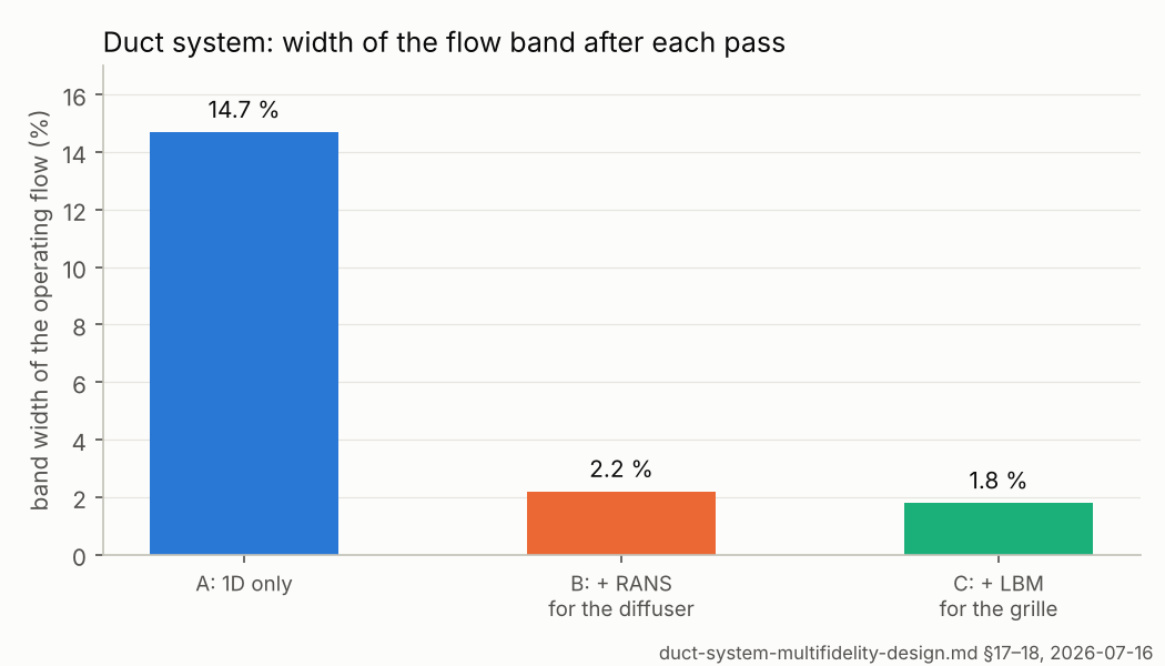
Duct system (fan, asymmetric diffuser, bend, grille in series, 2026-07-16). Each component gets its own tool: 1D everywhere, RANS for the separated diffuser, LBM for the grille that sheds vortices. The width of the operating-flow band falls from 14.7 % to 1.8 %, and the final flow is 0.13071 m³/s. The diffuser is also an honest miss: the RANS pressure recovery is 0.64–0.67 against 0.80 read from the reference figure.
Square cylinder (Lyn & Rodi, Re_D = 21,400, 2026-07-16). The 1D estimate gives St ≈ 0.13 and Cd 2.1. Steady RANS does not settle (Cd cycles between 2.8 and 3.1), so the question goes up. LBM with MRT and Smagorinsky sheds with St 0.1440 (+9.1 % against 0.132) and Cd 1.86 ± 0.12 (2.1 measured); with HRR the wake stayed steady and deflected.
Tee (2026-07-27). Solved with the handbook K, with K measured by LBM, and as a whole LBM: the error of the flow split falls from −0.0147 to −0.0004.
Cross ventilation (2026-08-30). 1D, OpenFOAM and LBM agree within about 3 % on the ventilation rate, and all three are about 70 % above the experiment of Tominaga & Blocken; eight candidate causes were tested and ruled out. See Cross ventilation.
Other cases with their own pages: Womersley pipe, LBM against FVM, swing jet, 1D arterial model.
Application: an apartment LDK
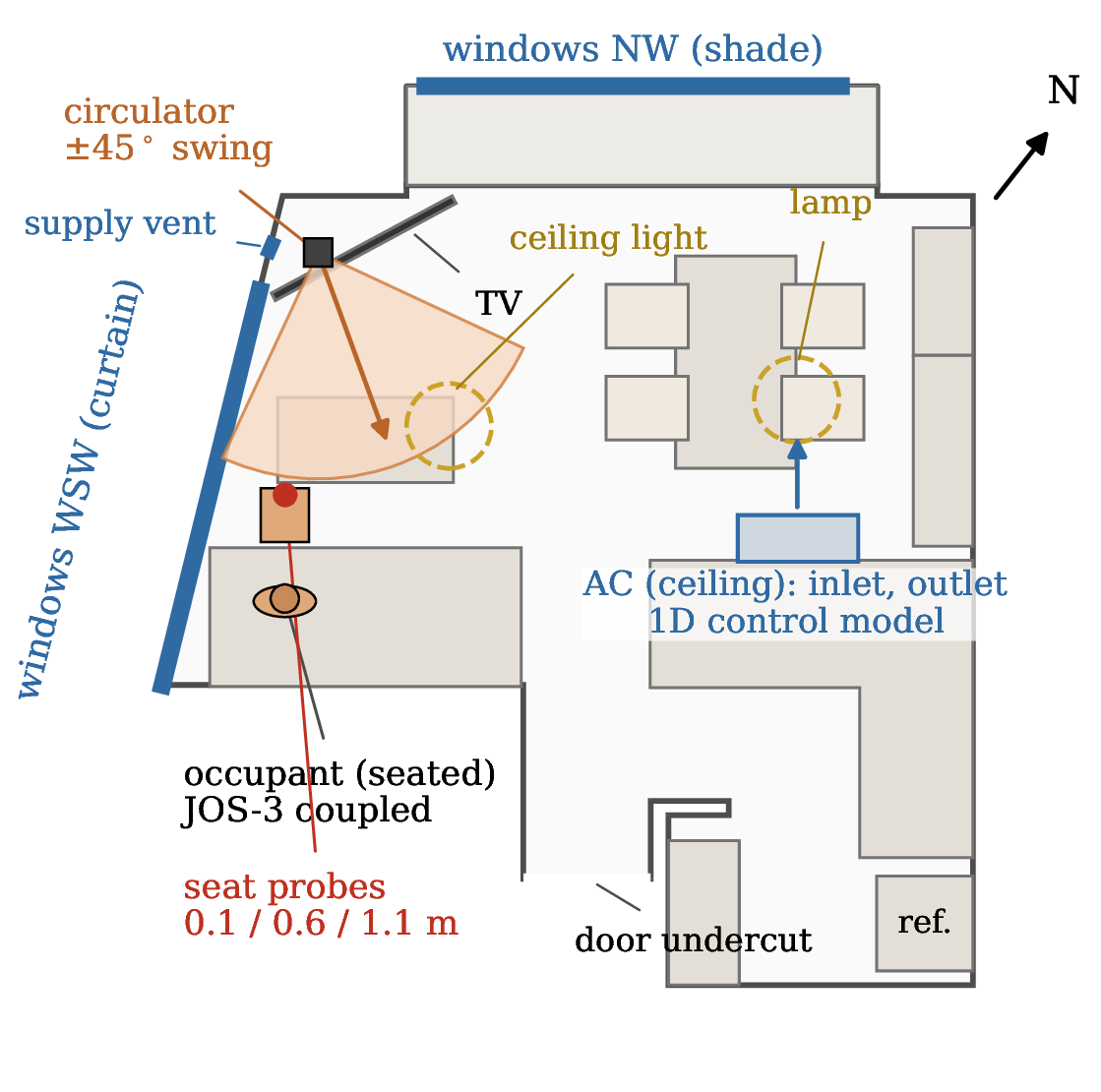
From the OpenCAE Symposium 2026 talk: the 1D model, steady FVM and unsteady LBM used on a real apartment LDK (living-dining-kitchen). The whole talk is summarised in OpenCAE Symposium 2026 talk.
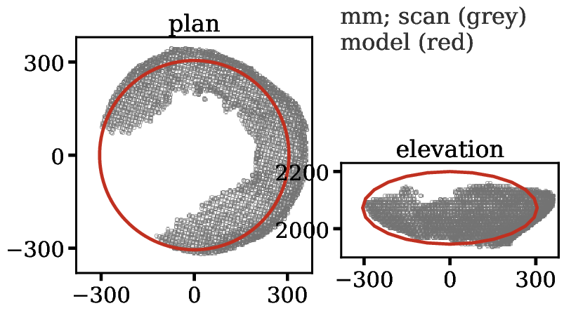
Target and measurements: mid-August, one adult seated on the sofa, air conditioner set to 27 °C. What the LLM asked to be measured was measured in turn: 53 surface temperatures (thermal camera) and 3 air temperatures (thermometer), 56 points in all. Geometry from the floor and furniture plans and a smartphone LiDAR scan. Metal surfaces and curtains were measured on black masking tape (glass reads 34.7–40.5 °C by reflection, 29.9–32.7 °C on the tape).
| Plan of the LDK | LiDAR scan (grey) and model (red) of a ceiling light |
|---|---|
 |
 |
Steady FVM coupled to 1D models:
| Item | Calibrated case |
|---|---|
| Solver | buoyantSimpleFoam with the radiation bug fixed |
| Mesh, iterations | about 1.25 M cells (48 ranks), 30,000 iterations |
| Turbulence | k-ω SST (Spalding wall function) |
| Radiation | viewFactor, 4,440 coarse faces, self-radiation included |
| Occupant | JOS-3 (83 nodes), coupled every 50 iterations |
| AC supply | 0.196 kg/s at 22.0 °C (proportional control) |
| Heat | 724 W gain / 946 W removed by the AC |
| Outdoor | 29.1 °C (AMeDAS) |
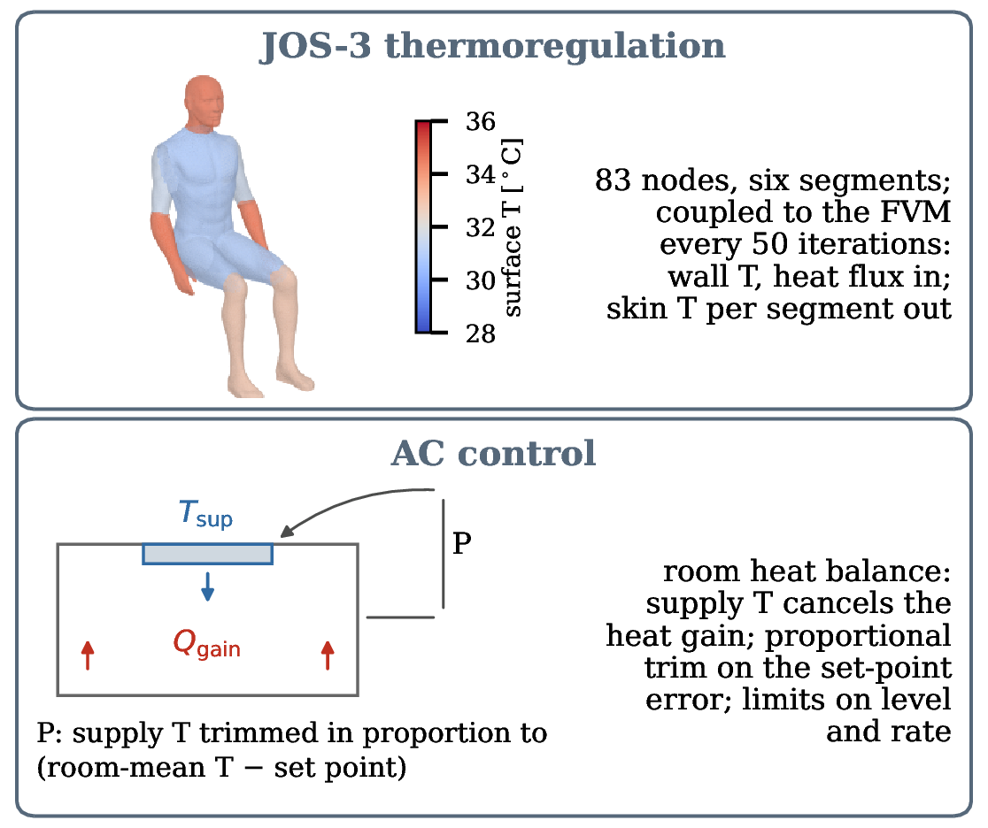
Coupling JOS-3 instead of fixing the skin temperature raises the body heat loss 37.4 → 51.0 W and lowers the heat-balance residual 157 → 129 W. Against the 56 measured points the RMS is 0.63 K (0.60 K not windows, 0.69 K windows); 13 of the 14 window points are computed low, by −0.55 K on average.
From FVM to LBM: LBM alone missed the near-floor flow of the cold falling supply air (0.02 and 0.05 m/s at 0.1 and 0.6 m against the FVM's 0.25 and 0.21 m/s). The steady FVM velocity and temperature were therefore mapped onto the LBM grid as a base state, held by a force and a heat source, and the LBM solved the fluctuation. Results: Swinging jet.
Still open
- The port of the Modelica Standard Library and the OpenModelica cross-check are in development and not yet in the public source (One-dimensional models).
- The K table of the laminar duct case still holds placeholder values.
- The backward-facing step: the pressure drop is not harvested from RANS yet.
- The laminar step solved three ways and coupled into one circuit (Armaly) was designed, not built.
- The model base (a sketch or prompt turned into a typed network) has only its network solver.
- The swing jet has no FVM half yet.
Design records
Frozen; they are not updated and are not translated.
- multifidelity-1d-design.md, onedim-validity-criteria.md, onedim-alpha-design.md, onedim-modelica-design.md — the 1D tier
- model-base-design.md — the model base
- steady-rans-rung-design.md — the steady RANS tier
- bfs-three-rung-design.md, mf-bfs-3tier-design.md — backward-facing step
- duct-system-multifidelity-design.md — duct system
- square-cylinder-design.md, cylinder-escalation-design.md — square and circular cylinder
- mf-tee-heated-design.md, validation-expansion-design.md — tee, heated duct and the MF series
- ladder-cases-design-2026-08.md — cross ventilation and the swing jet
- grand-showcase-design.md, showcase-cases-design.md — showcases
- hybrid-external-lbm-driver.md — driving OpenLB, Palabos and waLBerla