advection-diffusion2d
English | Japanese
« Home · « Advection-diffusion, reaction and radiation
Advection-diffusion of a passive scalar (2D Gaussian pulse) -- exact-solution verification benchmark. A single D2Q5 advection-diffusion LBM for the scalar C, advected by a PRESCRIBED UNIFORM velocity u = (U, 0) on a doubly-periodic square. The scalar is passive: there is no momentum LBM, no buoyancy coupling -- u is imposed everywhere, so this isolates the D2Q5 collision/streaming as a pure advection-diffusion operator and checks it against the textbook Gaussian Green's function.
Geometry
Animation
Fields
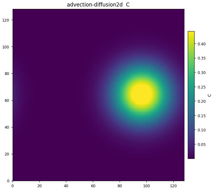
The fields this computation wrote at its last output step, plotted as they are. 3D cases show the mid-plane.
Results
A pure transport benchmark that validates a D2Q5 scalar LBM against an exact solution (the 2D Gaussian kernel). Default arguments: N = 128, lattice advection velocity U = 0.05, D_phys = 0.0064, T = 0.5, σ0 = 0.08. The mapping is D_lat = 0.0064 × 0.05 × 128 = 0.040960, τ = 3 × 0.04096 + 1/2 = 0.62288, steps = 0.5/(0.05/128) = 1280, and the Pe based on the pulse width is Pe = U σ0N/D_lat = 0.05 × 10.24/0.04096 = 12.5 — every number in the 1st line of the log closes with this arithmetic. Wall-clock time 1.11 seconds on 72 Grace CPU cores.
- L2 error first decreases from 1.7820e-03 (step 25) (minimum 1.3132e-03, around step 325) and ends at 1.8139e-03. Over the whole run it stays in the 1.3–1.8e-3 band.
- Growth of the variance: final σ² = 209.041 vs exact 209.715. The exact value is σ0² + 2 D_lat t = 104.8576 + 2 × 0.04096 × 1280 = 209.7152 — the run stops exactly at the time when the initial variance has doubled. The diffusion slope of the linear fit is 8.162253e-02, against the theoretical 2D = 2 × 0.04096 = 0.08192, i.e. −0.36%. Intercept 104.5727 vs σ0² = 104.8576.
- Advection velocity: centroid tracking gives 5.000004e-02 vs U = 0.05 (0.00%). Translation on the lattice is reproduced almost exactly by D2Q5.
- Conservation: M/M0 = 1.000000 at every step. Evidence that both collision and streaming conserve the total scalar to machine precision.
Governing equations
The advection–diffusion equation for a passive scalar C and its Green's function:
\[
\partial_t C + U\,\partial_x C = D\,\nabla^2 C,\qquad
C=\frac{\sigma_0^2}{\sigma^2}\exp\!\Big(\!-\frac{(x-x_0-Ut)^2+(y-y_0)^2}{2\sigma^2}\Big),\;
\sigma^2=\sigma_0^2+2Dt
\]
This is solved with BGK on D2Q5 (rest + 4 axis directions, w0 = 1/3, w1..4 = 1/6, c_s² = 1/3). The equilibrium distribution and the recovered diffusion coefficient:
\[
g_i^{\rm eq}=w_i\,C\Big(1+\frac{\boldsymbol{c}_i\cdot\boldsymbol{u}}{c_s^2}\Big),
\qquad D=c_s^2\Big(\tau-\tfrac12\Big)\;\Rightarrow\;\tau=3D+\tfrac12
\]
The velocity field u = (U, 0) is prescribed (no momentum LBM). In other words, this case isolates the D2Q5 collision and streaming as a pure advection–diffusion operator and checks it against the textbook Green's function. The exact solution is evaluated as a lattice sum over periodic images, so the reference side does not limit the L2 measurement. Fixing U per grid and raising N gives dx = 1/N and dt = U dx, so a 2nd-order-convergence grid-refinement test is well posed (see the header).
Code walkthrough
Source (363 lines).
%%{init: {'themeVariables': {'fontSize': '11px'}}}%%
flowchart LR
    subgraph DOM["Doubly periodic square lattice 128×128"]
      P(("Gaussian pulse σ0=10.24 cells<br/>translated by prescribed velocity u=(U,0)<br/>self-similar diffusion σ²=σ0²+2Dt"))
    end
DOM -->|periodic wrap x,y| DOM- Mapping — derive (D_lat, τ, steps) from (N, U, D_phys, T, σ0) and print them.
- collide/stream — D2Q5 BGK. The only boundary treatment is periodic array indexing.
- Diagnostics — every 25 steps, output the L2 (against the exact solution summed over periodic images), the second moment σ², and the total M/M0.
- Summary — slope of the straight-line fit of σ²(t) vs 2D, centroid velocity vs U, RESULT line.
Build & run
cmake -S native -B native/build && cmake --build native/build -j
./native/build/orheo-advection-diffusion2d
advection_diffusion2d [N] [U] [D_phys] [T] [sigma0] [out_prefix]
Cost of the computation that made the figures on this page (Miyabi-G Grace CPU (72 cores, -stdpar=multicore)): 1.1 s wall.
Things to try
- Grid refinement:
advection_diffusion2d 256→ 512. Since U is fixed, L2 should fall as dx². Measure the order of decay yourself. - The danger zone τ → 1/2: reduce D_phys to 1/10 and look at how the error behaves around τ = 0.512 (stable, but the error structure changes).
- Vary Ma: U = 0.05 → 0.2. Check whether contamination of 2nd order in the lattice Mach number appears in the advection-velocity error (0.00% in this run).
- Make σ0 smaller: narrowing the pulse to a few cells makes the numerical dispersion of D2Q5 visible. How much does the initial L2 value jump?
Validation
| Tier | T0 — order of convergence verified |
| QoI | temperature-L2-error(abs) |
| Reference | analytic Gaussian Green's function of the AD equation |
| Gate | 🧩 module gate (advection_diffusion) |
| Measured | 0.001813924 (rel. err +0.18%) — harvest N=128 |
Source & run details
| Item | Value |
|---|---|
| Target | orheo-advection-diffusion2d |
| Source | native/benchmarks/advection_diffusion2d.cpp |
| Lattice | D2Q5 |
| GPU twin | no |
| Gallery run | 2026-07-27 @ 7628c0cf |
| Args | `` |
| Wall time | 1.11 s |
| CPU time | 14.07 s |
| Device | Miyabi-G Grace CPU (72 cores, -stdpar=multicore) |
Computation log
The actual output of this computation (head and tail).
advection_diffusion2d N=128 U=0.0500 D_phys=0.0064 T=0.500 sigma0=0.080 | D_lat=0.040960 tau=0.62288 steps=1280  Pe=12.5
  step 25/1280: L2=1.7820e-03 sigma2=106.623 (exact 106.906) M/M0=1.000000
  step 50/1280: L2=1.6671e-03 sigma2=108.664 (exact 108.954) M/M0=1.000000
  step 75/1280: L2=1.5866e-03 sigma2=110.704 (exact 111.002) M/M0=1.000000
  step 100/1280: L2=1.5245e-03 sigma2=112.744 (exact 113.050) M/M0=1.000000
  step 125/1280: L2=1.4748e-03 sigma2=114.785 (exact 115.098) M/M0=1.000000
  step 150/1280: L2=1.4344e-03 sigma2=116.825 (exact 117.146) M/M0=1.000000
  step 175/1280: L2=1.4016e-03 sigma2=118.865 (exact 119.194) M/M0=1.000000
  step 200/1280: L2=1.3751e-03 sigma2=120.906 (exact 121.242) M/M0=1.000000
  step 225/1280: L2=1.3542e-03 sigma2=122.946 (exact 123.290) M/M0=1.000000
  step 250/1280: L2=1.3380e-03 sigma2=124.986 (exact 125.338) M/M0=1.000000
  step 275/1280: L2=1.3261e-03 sigma2=127.026 (exact 127.386) M/M0=1.000000
  step 300/1280: L2=1.3180e-03 sigma2=129.067 (exact 129.434) M/M0=1.000000
  step 325/1280: L2=1.3132e-03 sigma2=131.107 (exact 131.482) M/M0=1.000000
...

  step 1250/1280: L2=1.7975e-03 sigma2=206.594 (exact 207.258) M/M0=1.000000
  step 1275/1280: L2=1.8112e-03 sigma2=208.633 (exact 209.306) M/M0=1.000000
  step 1280/1280: L2=1.8139e-03 sigma2=209.041 (exact 209.715) M/M0=1.000000
--- N=128 summary ---
  L2(final)          = 1.8139e-03
  diffusion slope    = 8.162253e-02  vs 2D = 8.192000e-02  (-0.36%)
  sigma^2 intercept  = 104.5727  vs sigma0^2 = 104.8576
  advection speed    = 5.000004e-02  vs U = 5.000000e-02  (0.00%)
RESULT N=128 L2=1.813924e-03 slope=8.162253e-02 twoD=8.192000e-02 speed=5.000004e-02 U=5.000000e-02 sig2fit0=104.572694 sig0sq=104.857600
References
- R. G. M. van der Sman & M. H. Ernst, J. Comput. Phys. 160 (2000) 766 — D2Q5 diffusion lattice.
- X. He, S. Chen & G. D. Doolen, J. Comput. Phys. 146 (1998) 282 — advection–diffusion equilibrium distribution.