magnetic-particles2d
English | Japanese
« Home · « Particles and fluid-structure interaction
Magnetophoresis of a suspended magnetizable particle in an LBM flow. --------------------------------------------------------------------------- A weakly-magnetizable particle (a magnetic bead) suspended in a quiescent fluid feels a body force in a NON-UNIFORM external magnetic field and drifts up the field-energy gradient -- the physics of lab-on-a-chip bead separation, magnetic drug targeting and ferrofluid actuation (the OpenLB magneticParticles menu). In the linear point-dipole limit the magnetophoretic force is
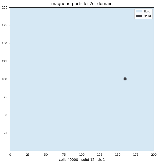
Geometry
Animation
Fields
The fields this computation wrote at its last output step, plotted as they are. 3D cases show the mid-plane.
Results
Magnetophoresis of magnetised beads drifting in the magnetic field of a straight current-carrying wire. 200×200 periodic box, D2Q9 BGK (τ = 0.8, μ = 0.1), wire at the centre (100, 100), beads with a = 2, Δχ = 1, K = 5, released from radius r0 = 60. The coupling is one-way (beads do not disturb the fluid): the particle response time is τ_p = 2a²ρ_p/(9μ) = 2×4/0.9 = 8.89 steps, Re_p = 0.041. Wall-clock 17.9 s on 72 Grace CPU cores.
The validation consists of 3 checks against the analytic solution u_mag (theory below), all accurate to sub-%.
- Trajectory: along the whole inward path from r0 = 60, |v_p(r)| is compared with the local u_mag(r). At the sample point r = 59.59, v = 1.0495e-3 vs analytic 1.0500e-3, error -0.05%.
- K sweep (a = 2 fixed, K = 2..6): errors -0.01% to -0.08%. It follows the u_mag ∝ K² scaling exactly (1.6513e-4 at K=2 → 1.5248e-3 at K=6).
- a sweep (K = 5 fixed, a = 1.5..3.5): errors -0.02% to -0.47%. u_mag ∝ a². Maximum error over all sweeps 0.47% (the closing line of the log).
The ends of the trajectory CSV need to be read honestly. The step 0 row has an error of -89.9% — just after release from rest; by step 100, when the τ_p ≈ 9 step relaxation is over, it falls to -0.05%. Conversely, near the wire the error grows again: -15.7% at r = 12.67 and -18.1% at the last row, r = 11.97. This is the region where u_mag ∝ 1/r³ changes substantially within the distance travelled in 1 step, and the quasi-steady (terminal-velocity) approximation breaks down. The valid validation interval is from after the release transient to a few wire radii short of the wire.
Governing equations
Balance between the magnetophoretic force in the linear point-dipole limit and Stokes drag in quiescent fluid:
\[
\boldsymbol{F}_m=\frac{V_p\,\Delta\chi}{\mu_0}(\boldsymbol{B}\cdot\nabla)\boldsymbol{B},
\qquad
u_{\mathrm{mag}}=\frac{F_m}{6\pi\mu a}
=\frac{2a^{2}\Delta\chi}{9\mu\mu_0}\,|(\boldsymbol{B}\cdot\nabla)\boldsymbol{B}|
\]
The external field is the true (curl-free/divergence-free) field of a straight current-carrying wire:
\[
\boldsymbol{B}=K\,\frac{(-y,\;x)}{r^{2}},\qquad K=\frac{\mu_0 I}{2\pi},\qquad
|(\boldsymbol{B}\cdot\nabla)\boldsymbol{B}|=\frac{K^{2}}{r^{3}}\ (\text{inward})
\]
At r0 = 60, u_mag = (2×4×1)/(9×0.1×1) × 25/60³ = 1.0288e-3 (matches the log).
Why a one-way-coupled point particle: in 2D there is no Stokes-drag limit (the Stokes paradox). Because the drag on a resolved 2D disk cannot be pinned to an analytic formula, a point particle that samples the flow velocity bilinearly from the LBM field and applies the 3D Stokes drag \(6\pi\mu a(\boldsymbol{u}_f-\boldsymbol{v}_p)\) gives a clean quantitative validation against the analytic solution (details in magnetic-particles-design.md). The fluid stays at rest, undisturbed. Equation of motion (neutrally buoyant, so gravity drops out):
\[
m_p\frac{d\boldsymbol{v}_p}{dt}=\boldsymbol{F}_m+6\pi\mu a(\boldsymbol{u}_f-\boldsymbol{v}_p),
\qquad m_p=\rho_p\tfrac43\pi a^{3}
\]
Code walkthrough
Source (405 lines).
%%{init: {'themeVariables': {'fontSize': '11px'}}}%%
flowchart LR
    subgraph BOX["200×200 periodic box · D2Q9 BGK · quiescent fluid"]
      W(("Wire<br/>(100,100)")) -. "B = K(-y,x)/r²" .-> P["Point bead<br/>Stokes drag + F_m<br/>u_f by bilinear interpolation"]
    end
P --> T["traj.csv / sweep.csv"]- Field evaluation — the wire field is evaluated analytically at the bead centre every step (not put on the grid).
- Particle update — semi-implicit Euler, dt = 1. Stops when r < rmin.
- Trajectory mode — follows 1 bead from r0 = 60, recording v and the local u_mag side by side at each sample.
- Sweep mode — 5 points in K and 5 points in a. At each point, the terminal velocity near a fixed r0 is measured and its error against the analytic value written to the CSV, 1 row per point.
- Two-way variant — write-back via a Guo body force exists in the code but is off by default (twoway key).
Build & run
cmake -S native -B native/build && cmake --build native/build -j
./native/build/orheo-magnetic-particles2d
Cost of the computation that made the figures on this page (Miyabi-G Grace CPU (72 cores, -stdpar=multicore)): 17.9 s wall.
Things to try
- Set twoway=1. How does the error move when the bead reaction is returned to the fluid via Guo forcing? For a point particle with a = 2 cells the effect should be small, which in itself confirms the validity of the one-way approximation.
- Raise a to 4, 6. Extrapolate the trend line of the error growth in the a sweep (-0.02% → -0.47%) and find the particle size at which the point-dipole approximation, "field gradient uniform over the particle", breaks down.
- Lower rmin and draw the near-field error curve. Plot err_pct vs r from traj.csv and check whether the radius at which the quasi-steady approximation breaks down matches the estimate from τ_p and 1/r³.
- Lower τ to 0.6. μ changes, so τ_p and u_mag both move. Seeing the analytic formula follow shows that the validation is not a coincidence of parameters.
Validation
| Tier | T2 — single-point comparison |
| QoI | Migration trajectory |
| Reference | Point-dipole force + Stokes drag (analytic) |
| Gate | — no gate |
Source & run details
| Item | Value |
|---|---|
| Target | orheo-magnetic-particles2d |
| Source | native/benchmarks/magnetic_particles2d.cpp |
| Lattice | D2Q9 |
| GPU twin | no |
| Gallery run | 2026-07-27 @ 7628c0cf |
| Args | `` |
| Wall time | 17.93 s |
| CPU time | 346.99 s |
| Device | Miyabi-G Grace CPU (72 cores, -stdpar=multicore) |
Computation log
The actual output of this computation (head and tail).
Magnetophoresis of a point bead in a wire field (D2Q9, one-way Stokes-drag point particle)
  grid 200x200  tau=0.800 mu=1.0000e-01  wire @ (100.0,100.0)  coupling=one-way
  bead a=2.00 dchi=1.00 mu0=1.00 K=5.00 rho_p=1.00  r0=60.0
  tau_p=8.89 steps  u_mag(r0)=1.0288e-03  Re_p=0.041
[trajectory] releasing bead at r0=60.0 ...
[trajectory] wrote ./magnetic_particles2d_traj.csv (sample r=59.59 v=1.0495e-03 ana=1.0500e-03 err=-0.05%)
[sweep K] a=2.00 fixed, K in {2,3,4,5,6}
  K=2.0  r=59.94  v=1.6513e-04  ana=1.6514e-04  err=-0.01%
  K=3.0  r=59.85  v=3.7301e-04  ana=3.7308e-04  err=-0.02%
  K=4.0  r=59.74  v=6.6684e-04  ana=6.6706e-04  err=-0.03%
  K=5.0  r=59.59  v=1.0495e-03  ana=1.0500e-03  err=-0.05%
  K=6.0  r=59.41  v=1.5248e-03  ana=1.5260e-03  err=-0.08%
[sweep a] K=5.00 fixed, a in {1.5,2,2.5,3,3.5}
  a=1.5  r=59.77  v=5.8532e-04  ana=5.8542e-04  err=-0.02%
References
- M. A. M. Gijs, "Magnetic bead handling on-chip", Microfluid. Nanofluid. 1 (2004) 22–40.
- N. Pamme, "Magnetism and microfluidics", Lab Chip 6 (2006) 24–38.
- E. P. Furlani, "Analysis of particle transport in a magnetophoretic microsystem", J. Appl. Phys. 99 (2006) 024912.