One-dimensional models
English | Japanese
The one-dimensional models are the first of OpenRheo's three levels. They solve a whole system on one CPU core in under a second. Each model also reports whether its result is inside the range where it can be trusted. This page describes the public models and their checks, when a question moves up a level, and the port of the Modelica Standard Library that is in development.
Place among the three levels
A question is answered by the cheapest level that can answer it. The levels, from cheapest, are the 1D models, steady FVM (RANS in OpenFOAM) and unsteady LBM. A fixed rule, not the LLM, decides whether a question moves up. The rule and the cases taken up the ladder are on Multi-fidelity.
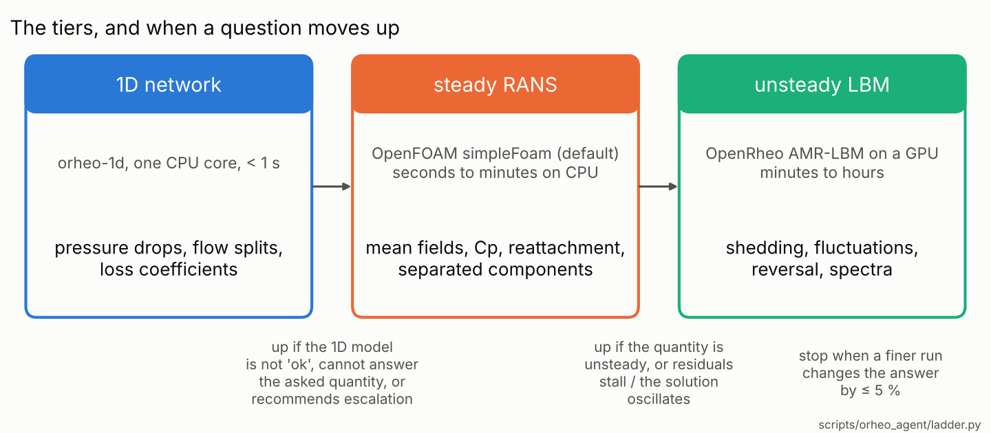
The decision has two parts. The first is "is 1D enough?". It is enough when the parameters are inside the model's range and the requested quantity is not on the model's cannot_answer list. The second is "is the flow inherently unsteady?". Each model carries an onset criterion for unsteadiness, such as a Reynolds number.
| Is 1D enough? | Unsteady? | Level |
|---|---|---|
| yes | below onset | stop at 1D; quote the error band |
| yes | above onset, only mean values asked | stop at 1D; keep a warning that the flow is unsteady |
| no | steady, little separation | steady FVM; the measured loss coefficient K goes back into 1D (k_custom) |
| no | a fluctuation quantity (spectrum, peak) is asked, or a separated bluff-body wake | skip steady FVM and go to LBM |
A steady FVM stage is not connected to a flow that is not steady: steady RANS does not converge there, and it does not give fluctuation quantities at all. The 1D level can say that a flow sheds vortices, and roughly at what frequency. It cannot give the amplitude or the waveform.
Running it and its output
The 1D level is one program, orheo-1d (orheo_1d.cpp). Its input is a list of KEY=VALUE pairs, on the command line or in a file.
orheo-1d model=duct given=dp dp=5e4 L=10 D=0.05 eps=4.5e-5 K=entrance,exit
orheo-1d model=crossvent A=0.9 Cp_in=0.7 Cp_out=-0.3 U=3 V=62.5 A_wall=12
The output is a CSV for plotting and a summary.json. The summary.json has a fixed schema, openrheo-1d-summary/1, and the LLM agent reads it instead of the standard output (summary_json.hpp). Its main fields:
| Field | Content |
|---|---|
qois |
the computed quantities, with values and units |
status |
ok, marginal or invalid; it only ever moves down |
flags |
marks for out-of-range inputs and assumptions (e.g. transitional_re, porosity_above_orifice_model_limit) |
expected_error_band |
the expected size of the error |
cannot_answer |
quantities this model cannot give |
escalate |
whether a higher level is recommended, and why |
suggest_3d |
cells, steps and an estimated GPU time for the higher level |
summary.json is written even when the input is invalid, so the agent never faces a level that stopped silently. The GPU time is estimated from measured GPU throughput (cost_model.hpp). It is an estimate only.
The models
The source is in native/include/openrheo_amr/onedim/. The checks are ctests in native/tests/.
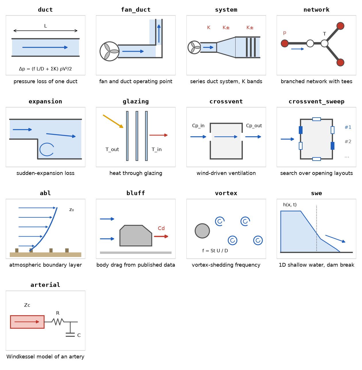
The figure above sketches what each model describes. It shows concepts, not results.
model= |
Role | Main inputs → outputs | Checked against (ctest) |
|---|---|---|---|
duct (duct.hpp) |
pressure loss of one duct | length, diameter, roughness, fitting K, Δp or flow rate → flow rate or Δp, friction factor, Re | laminar f = 64/Re; a Moody-chart value (f = 0.0222 ± 2 % at Re = 10⁵, ε/D = 10⁻³); the fully rough limit; the inverse round trip (test_duct1d) |
fan_duct (fan_duct.hpp) |
operating point of a fan and a duct | shut-off pressure, maximum flow, number of bends, K → operating flow rate and Δp | the intersection of the two curves; the dependence of bend K on R/D and Re; the shift of the operating point with a measured K (test_fanduct1d) |
system (duct_system.hpp) |
a series duct system | a list of components, each K a value or a band → flow-rate band, contribution of each component | equal to fan_duct to 10⁻¹⁰; conversion of the K reference velocity; propagation of the bands (test_duct_system1d) |
network (network.hpp, junction.hpp) |
a branched network; tees from Idelchik ch. 7 | nodes (fixed-pressure plenums, junctions), edges (ducts, fans, tees) → node pressures, edge flows | the conversion between K definitions is exact; a K that cannot be converted is refused by name (test_network_k_convention) |
expansion (expansion.hpp) |
sudden-expansion loss (Borda–Carnot) | expansion ratio, step height, velocity → K, static-pressure recovery | K₁ = 1/9, K₂ = 1/4, Cp = 4/9 at expansion ratio 1.5, to 10⁻¹²; the Borda limit (test_expansion1d) |
glazing (glazing.hpp) |
heat transfer through glazing, and the room-side surface temperature | number of panes, gap widths and gases, outdoor and room temperatures, solar → U, solar heat gain coefficient, surface temperatures, condensation | the analytic solution; the heat-flux balance; EN 673 centre-of-glass U for four build-ups (5.7 to 0.7 W/m²K); the solar balance (test_glazing1d) |
crossvent (crossvent.hpp) |
wind-driven ventilation rate | opening areas and discharge coefficients, pressure coefficients Cp, wind speed, room volume → ventilation rate, air changes per hour, direction | the series combination; the cancellation of density; the sign under reversed flow; the inverse round trip (test_crossvent1d) |
crossvent_sweep (crossvent_sweep.hpp) |
search over opening layouts | Cp per face (from FVM), faces that may be opened, range of opening count and area → ranked layouts | equal to solving each layout directly; independent of the thread count (test_crossvent_sweep) |
abl (abl_column.hpp) |
neutral atmospheric boundary layer | roughness length z₀, wind speed at a reference height → wind profile, friction velocity, power-law exponent | the log law within 1 %; for the AIJ case A inflow, exponent 0.24 to 0.30 and 4.491 m/s at z/b = 2 within 5 % (test_abl1d) |
bluff (bluff_body.hpp) |
drag of a body, looked up from published data, not computed | shape class, velocity, viscosity, area, slant angle → Cd, Cl (Ahmed body only) | the table of Ahmed et al. (1984), Cd 0.285 at 25° slant; the Re regimes of spheres and cylinders (test_bluff1d) |
vortex (vortex_shedding.hpp) |
vortex-shedding frequency of circular and square cylinders | velocity, diameter, viscosity → St, frequency, Cd band | St = 0.198 (1 − 19.7/Re) for a circular cylinder at 47 ≤ Re ≤ 190; the regime flags (test_vortex1d); St 0.13 for the square cylinder from Okajima and Lyn et al. |
swe (swe1d.hpp) |
1D shallow water (dam break) | initial water level, bed, number of cells → depth and velocity in time, front position | the exact Ritter and Stoker solutions; a lake at rest stays at rest; depth stays non-negative; convergence order 1.5 or more; the gap to the Koshizuka experiment is recorded (test_swe1d) |
arterial (arterial.hpp) |
Windkessel model of one aortic segment | mean pressure, heart rate, cardiac output, radius, wall → pulse pressure, wave speed, Womersley number | exact limits and textbook ranges (test_arterial); not compared with measured waveforms. 1D arterial model |
The schema of summary.json itself is checked by test_1d_schema. This test runs the real orheo-1d on constructed inputs and checks that the expected flags are raised.
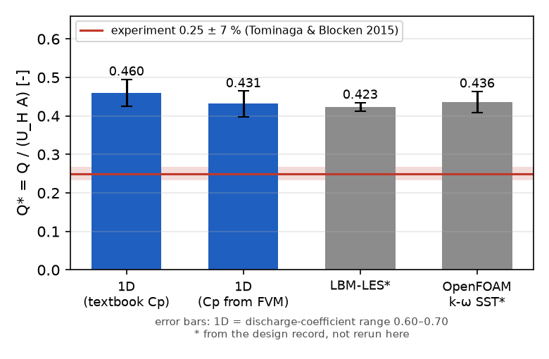
Most references are exact solutions, published values and internal consistency. Few models are compared directly with experiments. crossvent gives a ventilation rate about 70 % above the experiment (Tominaga & Blocken); LBM and OpenFOAM give the same value. Details are on Cross ventilation.
Example results
The figures below come from running orheo-1d from the public source (origin/main). Black and red are references; blue is the model.
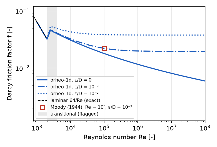
duct: friction factor against Re (the moody_sweep=1 output), with the laminar 64/Re line and the Moody value (f = 0.0222 at Re = 10⁵, ε/D = 10⁻³). In the grey transition range transitional_re is raised.
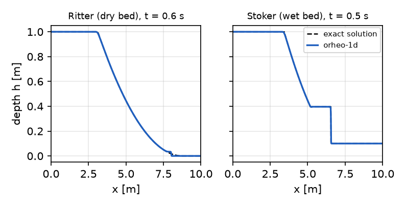
swe: dam break on 1000 cells. Left: dry bed (Ritter's exact solution). Right: wet bed (Stoker's exact solution). On the dry bed there is a small difference near the front.
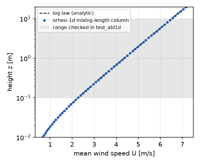
abl: the mixing-length column against the analytic log law (z₀ = 0.01 m, 5 m/s at 2 m). In the grey range test_abl1d checks that they agree within 1 %.
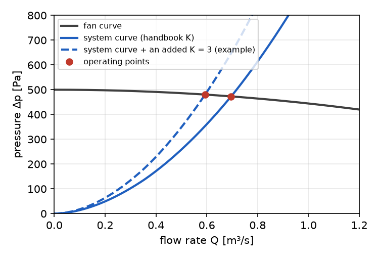
fan_duct: the operating point is where the fan curve meets the system curve (100 m long, 0.3 m diameter, 4 bends). Adding K = 3 moves it from 0.70 to 0.59 m³/s. The figure shows how the point is found; it is not a comparison with external data.
crossvent: the dimensionless ventilation rate Q* against the experiment (Tominaga & Blocken). The two 1D bars were run here; the LBM and OpenFOAM values are copied from the design record. All methods are about 70 % above the experiment, and the cause is not known.
An LLM wrote netlists from plain-language requests alone and solved all 10 tasks correctly: see 1D models built by an LLM from text.
Valid ranges and flags
Each model has a "card" that states its range (onedim-validity-criteria.md). A card lists the assumptions, the valid range, how the model fails, the onset of unsteadiness and the level to use instead. Outside the range, a flag is raised in summary.json.
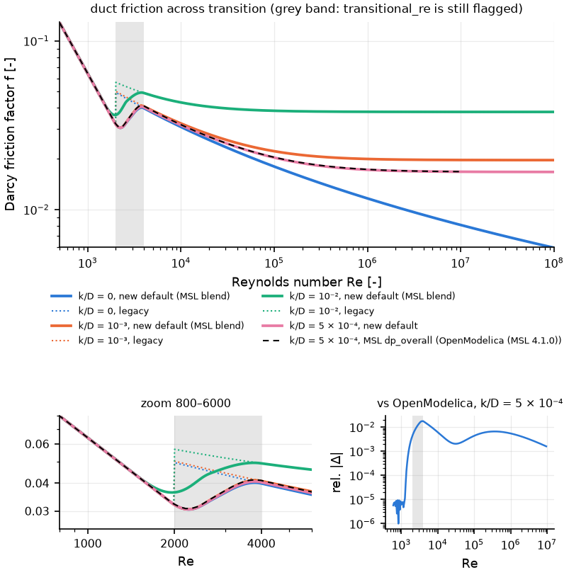
- Duct: laminar flow (Re < 2000) is exact with f = 64/Re. Turbulent flow (Re > 4000) uses Colebrook–White. In the transition between them,
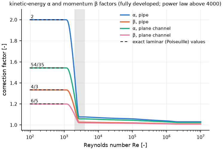
transitional_reis raised. In laminar flow the 1D bulk-velocity assumption itself fails: inventuri3d, the bulk-velocity Bernoulli Δp was 46 % below the measured pressure difference (the measured value is 1.86 times the formula), because the effect of the velocity profile (α ≈ 2) is missing. The development version adds α, which brings the difference to +7 %. - Tees and component K: handbook values have a band. A component whose band alone moves the system flow rate by more than 3 % is flagged as needing a measured K. The K is measured with steady FVM and goes back into 1D.
- Cross ventilation: above 10 % wall porosity the orifice model does not hold (Karava et al. 2011), and
porosity_above_orifice_model_limitis raised. The layout search takes such layouts out of the ranking and lists them for the higher level. - Drag and vortex shedding: both are correlations, not simulations. The flag
correlation_estimate_not_simulationis always raised. Flags are also raised at the drag crisis and at the transition to 3D flow. - Glazing:
condensation_on_indoor_glassis raised when the room-side glass condenses. - Atmospheric boundary layer: neutral stratification only; this flag is always raised.
For a component or range with no card, no advice is given. A higher level is recommended and a person is asked to decide.
In development: port of the Modelica Standard Library
In development
This section describes work in development. It is not in the public source yet (as of 2026-11-20; it is on development branches). The numbers are the results of the checks on those branches.
Approach
Modelica is a language in which components are written as equations and joined through connectors. OpenRheo does not build a Modelica compiler. The components of the Modelica Standard Library (MSL) 4.1.0 are rewritten as C++ libraries and assembled on one shared DAE (differential-algebraic equation) core. A component has connectors that pair a potential variable (temperature, voltage, ...) with a flow variable (heat flow, current, ...). A connection makes the potentials equal and the flows sum to zero. The code is header-only, with no dependency beyond the C++20 standard library. Results come out in the same summary.json form as the current level.
Licences
- MSL 4.0.0 and later are under the 3-clause BSD licence, so they can be ported into Apache-2.0 OpenRheo. Each ported component names its original class path and version in its header comment. The licence text is in
THIRD_PARTY_NOTICES.md. - MSL 3.2.3 and earlier are under a different licence (Modelica License 2) and are not ported.
- The Modelica Buildings library (LBNL) is under the 3-clause BSD licence with an added clause that licenses improvements back to LBNL. Version 15.0.0 is ported the same way, with attribution. What has been ported is listed under "Done" below.
- OpenModelica is used only as a tool to make reference data. OpenRheo does not need it to build or run.
How it is verified
For each package, the MSL examples are solved in C++ and compared with reference solutions. The reference solutions are made with OpenModelica and stored in the repository as small CSV files, with a record of how they were made. All reference solutions of the finished parts were made with OpenModelica 1.27.1 and MSL 4.1.0 (2026-11-20). Those of the thermal part used DASSL at tolerance 10⁻⁸.
While checking the port, we found six places where the MSL 4.1.0 code disagrees with its documentation or the standard. OpenRheo's default is the corrected behaviour. Details: Inconsistencies found in the Modelica Standard Library 4.1.0.
Done
Only representative figures are shown here. All figures are in the one-dimensional gallery.
Media, control blocks, tables and simple HVAC components
| Package | Content | Result |
|---|---|---|
Modelica.Media (MoistAir, DryAirNasa, liquid water) and psychrometrics |
saturation pressure, enthalpy, density, dew point, wet bulb, mixing | 13 quantities over 230 to 380 K against OpenModelica: relative error 10⁻¹² or less. Saturation pressure within 0.005 % of the ASHRAE table |
Modelica.Blocks (PID, LimPID, first order, limiter, hysteresis, ...) |
blocks in state-space form | the 6 states of the PID_Controller example within 0.001 % of their range; SlewRateLimiter within 7 × 10⁻⁵ |
Modelica.Blocks.Tables (CombiTable1D, CombiTimeTable) |
6 interpolation kinds (linear, Akima, ...), extrapolation, periodic tables | 22 models of ModelicaTest.Tables: relative error 5 × 10⁻⁸ or less |
| simple HVAC components (cooling coil, humidifier, mixing box) | not an MSL port; textbook equations | analytic checks (heat and moisture balances, saturation at the wet-bulb temperature) |
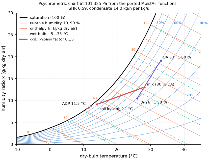
The psychrometric chart below is drawn only with the ported MoistAir functions. It carries a cooling-coil process: outdoor and return air mixed, then cooled to the leaving state on the line to the apparatus dew point (ADP), bypass factor 0.15.
The six states of the PID_Controller example against OpenModelica. Colour: OpenRheo; black dashed: OpenModelica. The deviation is at most 8.7 × 10⁻⁶ of the largest value.
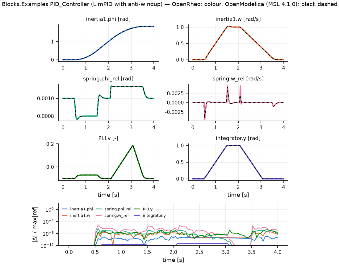
More figures are in the one-dimensional gallery.
Full media (IF97 water and steam, ideal gases, refrigerant, liquids)
| Package | Content | Result |
|---|---|---|
Modelica.Media.Water (IAPWS-IF97) |
regions 1 to 5, saturation, inverse functions, transport properties | all 227 entries of the IAPWS verification tables match |
Modelica.Media.IdealGases |
1241 species and mixtures from the NASA coefficients | relative error against OpenModelica 10⁻¹⁵ to 10⁻⁷ |
Modelica.Media.R134a, Air.ReferenceAir, liquids |
refrigerant R134a, the reference air equation of state, incompressible liquids | the same; R134a saturation also checked against the ASHRAE table |
The default is IAPWS-correct; a setting reproduces MSL 4.1.0 exactly (findings). In the figure below, the saturated-vapour enthalpy of water differs from OpenModelica by 4.6 × 10⁻⁸ with the default and by 2 × 10⁻¹⁴ with the MSL setting.
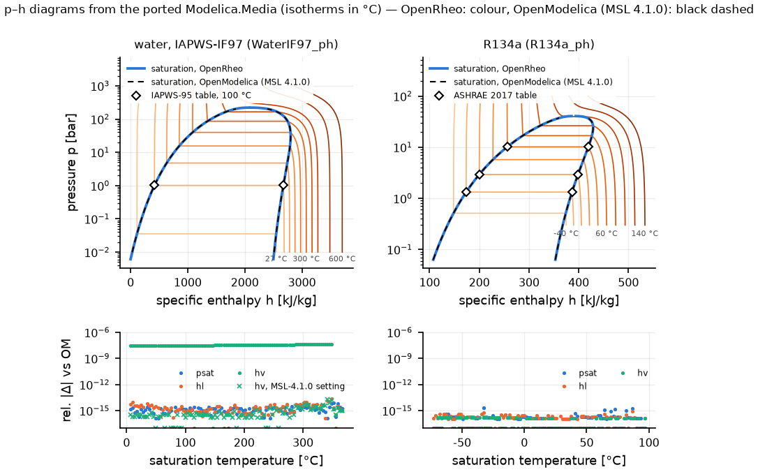
More figures are in the one-dimensional gallery.
Shared DAE core
| Package | Content | Result |
|---|---|---|
| DAE core | variable-order BDF (orders 1 to 5), index-1 DAEs, time and state events, initialisation and steady state, sparse LU | observed orders 0.99, 2.01, 3.03, 4.04, 5.06; Robertson within 4 × 10⁻⁷ of the reference at t = 40; van der Pol (μ = 1000) period within 2 × 10⁻⁵ of the asymptotic formula |
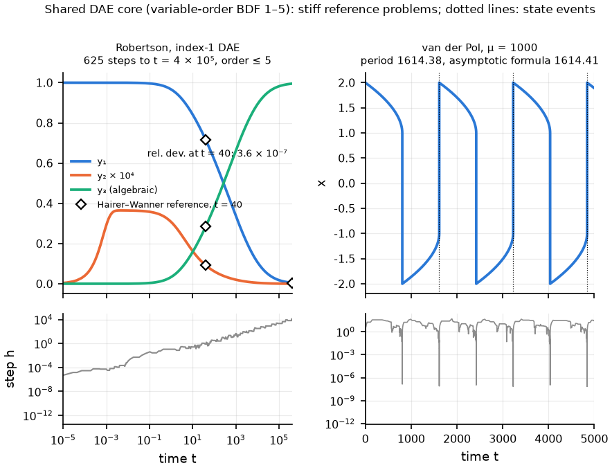
More figures are in the one-dimensional gallery.
ODE integration, heat-transfer network, multilayer wall, room heat balance
| Package | Content | Result |
|---|---|---|
| integrator | RK45, BDF1, BDF2; time and state events | orders 5.26, 1.00, 1.98; bouncing-ball impact times within 1.1 × 10⁻¹² s of the exact values |
Modelica.Thermal.HeatTransfer |
heat capacitors, conduction, convection, radiation, sources, sensors | difference from OpenModelica: TwoMasses example 1.4 × 10⁻⁵ K; Motor (RK45) 3.9 × 10⁻⁶ K (core), 2.2 × 10⁻⁵ K (winding); ControlledTemperature: all 18 switches match, largest time difference 1.4 × 10⁻⁵ s, largest temperature difference 8.4 × 10⁻⁵ K |
| multilayer wall | transient finite-volume conduction | 2.8 × 10⁻³ K from the Fourier-series solution (10 K step); spatial order 2.01 |
room heat balance and orheo-1d-room |
one well-mixed room; walls, window (via glazing), ventilation, heating and cooling |
2 × 10⁻⁹ K from the analytic adiabatic box; energy balance over 10 days 2 × 10⁻⁷ |
interior radiation exchange (Buildings InfraredRadiationExchange) |
grey radiation exchange between surfaces; the room default | with the Buildings view factors it reduces exactly to one star node; matches the full radiosity solve to 7 × 10⁻¹⁴ |
| wall layer division (Buildings rule) | number of cells per layer from the material data; optional | gives 3 cells for 0.2 m of concrete |
The TwoMasses reference solution is itself 1.4 × 10⁻⁵ K from the analytic solution; the C++ solution matches the analytic solution to 6.9 × 10⁻⁹ K.
ControlledTemperature switches 18 times under on/off control. The temperature and the switching are shown against OpenModelica.
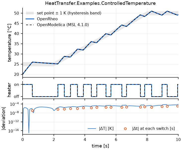
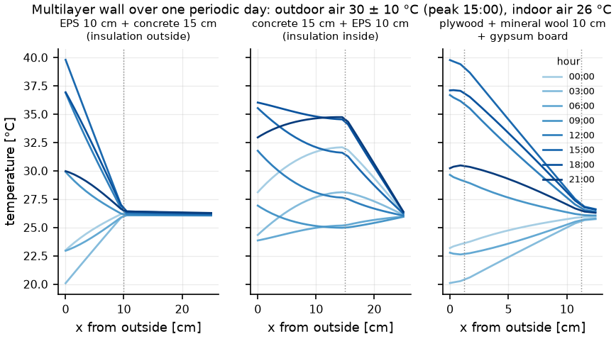
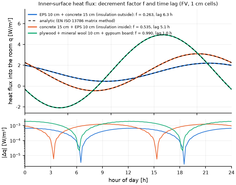
A multilayer wall under a daily outdoor cycle (30 ± 10 °C). The first figure shows the temperature inside the wall. The second shows the heat flux into the room against the analytic solution of the EN ISO 13786 matrix method; the decrement factors differ by 0.07 % or less and the time lags by 7 s or less.
The following parts of the Buildings library are not ported: windows (angle-dependent optics, shades, frame), states on the wall surfaces, phase-change materials, the exterior and sky radiation models, and geometric view factors. The example room (one room of an apartment) shows how the model behaves; it is not compared with measurements.
More figures are in the one-dimensional gallery.
Fluid networks
| Package | Content | Result |
|---|---|---|
Modelica.Fluid.Dissipation |
pressure loss of bends, orifices, straight pipes, channels of several cross-sections, valve geometries | relative error against OpenModelica 3 × 10⁻¹⁴ or less |
Modelica.Fluid.Machines |
pump and fan characteristics, affinity laws, efficiency and power | the same (including extrapolation at both ends of the curves) |
Modelica.Fluid.Valves |
Kv and Cv, valve characteristics, compressible flow, choking, leakage | defining equations and analytic checks |
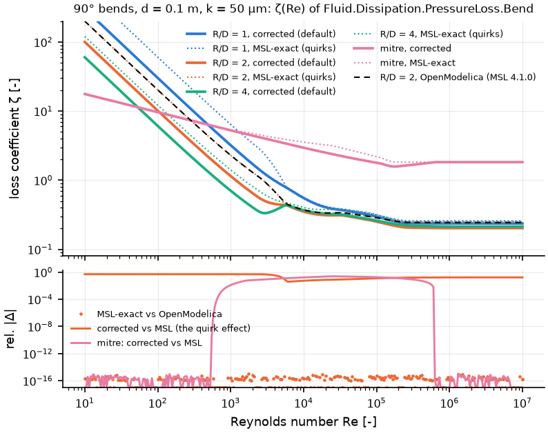
These components can be used as edges of the network solver (network). In three places the MSL code does not match its documentation and the literature: the laminar bend factor, the roughness scaling in the bends, and the valve Cv conversion factor. OpenRheo's default follows the documentation and the literature. A setting that reproduces MSL exactly is kept, and the comparison above uses it.
The bend K in duct and fan_duct becomes the MSL K(Re); the old table values can still be selected. The fan_duct figure above shows the current public source.
Bend loss coefficient ζ(Re), corrected default (solid) and MSL-exact setting (dotted). The MSL-exact setting matches OpenModelica to 1 × 10⁻¹⁵. The corrected default is half of MSL's value in laminar flow and up to 17 % lower at high Re.
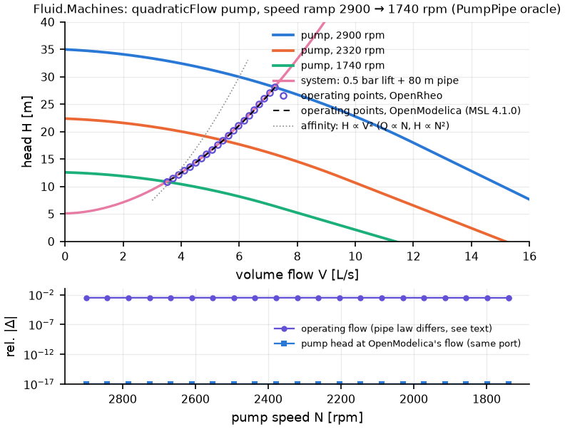
Pump curves, the system curve and the operating points over a speed ramp. The pump head matches OpenModelica exactly. The operating flow differs by 0.31 %, because the pipe laws differ (MSL WallFriction.Detailed, OpenRheo Dissipation.StraightPipe).
The duct friction factor now uses MSL's smooth transition. The old law jumped by 54 % at Re = 2000. Above Re = 4000 it is still Colebrook, up to 1.7 % from MSL's formula.
Where the area changes, the section-mean model uses the kinetic-energy factor α and the momentum factor β.
More figures are in the one-dimensional gallery.
Multibody systems
| Package | Content | Result |
|---|---|---|
Modelica.Mechanics.MultiBody |
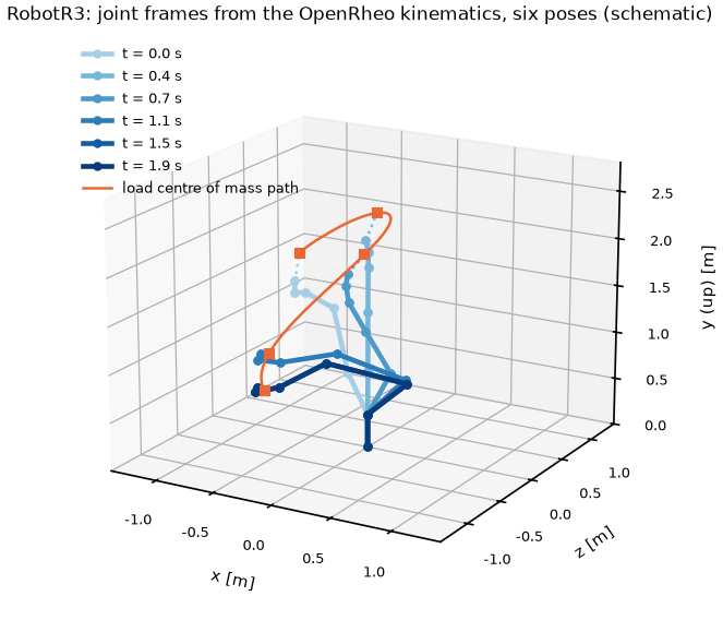
frames, parts, joints and constraint joints, gears, rolling wheels, forces, sensors; solved as a tree, with closed loops handled by cut-joint constraints | 37 examples agree with OpenModelica to about 10⁻⁷ to 10⁻⁹ (largest 1.6 × 10⁻⁵, in a chaotic example); energy conservation is checked (10⁻⁸ to 10⁻⁷ relative); RobotR3 inverse-dynamics torques match to 8 × 10⁻⁹ N m |
Modelica.Mechanics.Translational, Rotational |
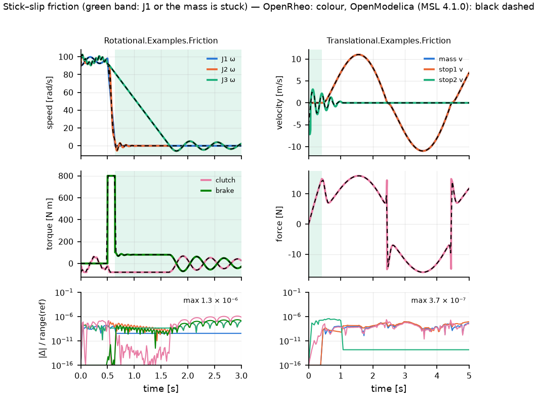
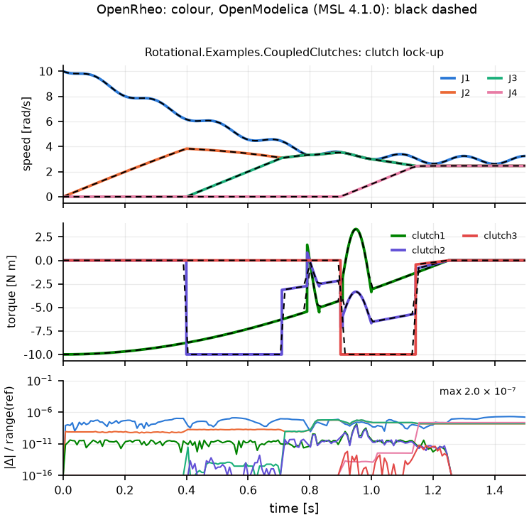
masses, inertias, springs, dampers, gaps, friction, clutches, brakes, lossy gears, vehicle | 27 examples within 3.6 × 10⁻⁵ of the value range of OpenModelica; 20 analytic checks; stick-slip handled with events |
The chaotic examples (BevelGear1D, ForceAndTorque, PointGravityWithPointMasses) are compared only up to t = 0.5 s, 3 s and 2 s. After that, even the OpenModelica result depends on the solver tolerance.
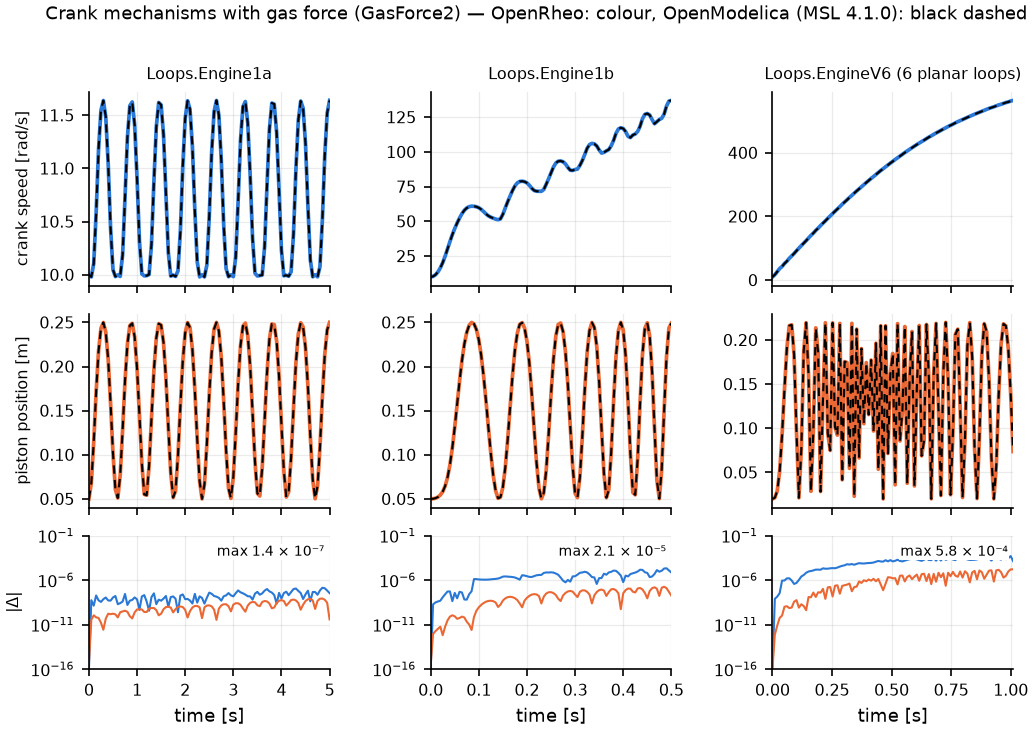
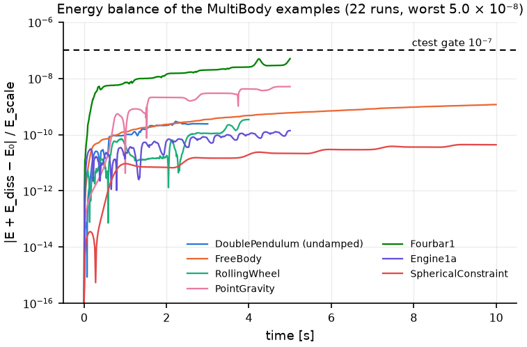
The first figure below is a schematic of RobotR3: the joint positions from the OpenRheo kinematics in six poses. Then three crank mechanisms driven by gas force (largest deviation 5.8 × 10⁻⁴ in EngineV6, at 565 rad/s), and the energy balance (at most 5 × 10⁻⁸ over 22 runs).
Stick-slip friction (green band: stuck) and clutch lock-up. The deviations are at most 1.3 × 10⁻⁶ and 2 × 10⁻⁷ of the value range.
The remaining classes are being ported.
Fluid heat flow and magnetic circuits
| Package | Content | Result |
|---|---|---|
Modelica.Thermal.FluidHeatFlow |
heat carried by fluid: pipes, pumps, valves, tanks, heat exchange | all non-example classes ported; against the OpenModelica examples, temperatures within 7 × 10⁻⁶ (of the largest temperature) |
Modelica.Magnetic.FluxTubes |
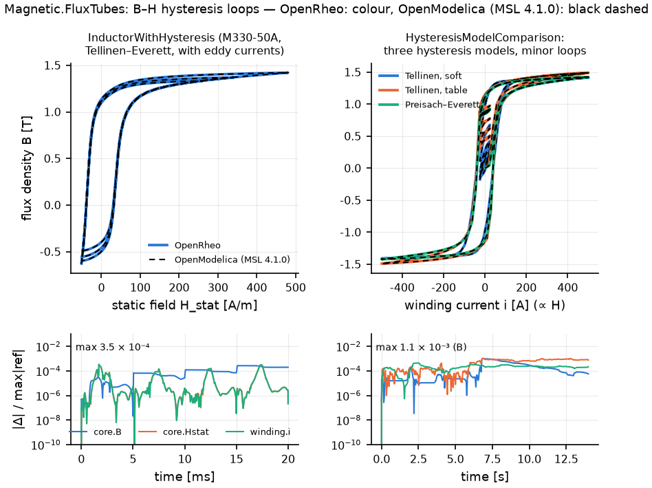
magnetic circuits: flux-tube shapes, leakage, force, hysteresis (Tellinen, Preisach), material data | the same; deviations about 10⁻³ or less, hysteresis included |
The two packages are compared on 34 OpenModelica examples. One ModelicaTest case (flux-tube force) differs by 4 × 10⁻³. This comes from the reference's own tolerance: an independent RK4 run matches OpenRheo to 10⁻⁹.
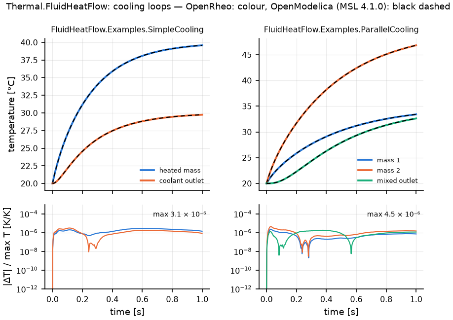
More figures are in the one-dimensional gallery.
Electrical circuits
| Package | Content | Result |
|---|---|---|
Modelica.Electrical.Analog |
basic and ideal elements, semiconductors (diode, MOSFET, transistor, thyristor, triac), 32 sources, sensors, transmission lines | 57 analytic checks and 38 OpenModelica examples plus 2 switching-time checks all pass; deviation 1e-16 to 8e-5 of the signal range |
Modelica.Electrical.Batteries |
cell stacks (CellStack, CellRCStack) and the discharge/charge example | voltage within 2.8e-6; remaining classes in progress |
The AD/DA converters and some examples are not ported yet. Ten cases (rectifier, thyristor and others) do not yet run on the shared DAE solver and use a test-only solver; the shared solver's event handling is being fixed.
Fluid components, electrical machines, math/logic and netlist (integrated 2026-11-22)
| Package | Content | Result |
|---|---|---|
Modelica.Fluid (vessels, pipes, heat exchangers, valves, pumps) |
ClosedVolume, OpenTank, DynamicPipe, StaticPipe, BasicHX, EquilibriumDrumBoiler, ValveDiscrete and stream connectors |
All ctests pass, including EmptyTanks, ThreeTanks, IncompressibleFluidNetwork, BranchingDynamicPipes, HeatExchangerSimulation, PumpingSystem, DrumBoiler, HeatingSystem and ControlledTanks |
Modelica.Electrical.Polyphase / Machines / PowerConverters |
polyphase, DC/induction/synchronous machines, transformers, rectifiers, inverters, choppers, batteries (CCCV_Cell, SuperCap) |
23 OpenModelica examples (14 on shared DAE core, 9 on fallback) + 92 analytic checks + independent closed-form validation (RLC resonance, DC motor, induction machine torque–slip) all pass |
Modelica.Math / ComplexMath / StateGraph / Clocked |
special functions, matrices, eigensolvers, distributions, RNG, FFT, complex blocks, StateGraph, periodic Clocked |
419 math checks, 17 complex functions, 6 StateGraph examples, 20 Clocked elementary examples + discrete controller all pass |
Plain-text netlist (orheo-1d model=msl) and independent validation |
builds and runs systems from text netlists emitting summary.json; 5 independent validation suites (IVP test set, wall conduction, water hammer, multibody, electrical) |
Netlist regressions (5 MSL reproductions + 28 negative tests + 8/10 LLM first-try evaluation) and the full 1D/MSL integration ctest suite pass 70 / 70 (-LE slow, 29.1 s) |
In progress and planned
The 1D integration branch (onedim-msl-integration) now passes 70/70 non-slow ctests. Remaining structural work and follow-ups:
- Move
MultiBody,FluidHeatFlow,FluxTubesand the thermal ODE path onto the shared DAE core for direct multi-domain coupling - Index-2 support, analytic Jacobians and AMD sparse ordering in the shared DAE core
- Remaining component registrations in the netlist and merge into the public
mainbranch
Design records
Frozen records, kept in English.
- multifidelity-1d-design.md — the 1D level and the
summary.jsoncontract - onedim-validity-criteria.md — the card of each model and the table that picks the level
- onedim-modelica-design.md — the strategy for using Modelica and the licence study
Related pages: Multi-fidelity, Multi-fidelity cases (1D ⇄ FVM ⇄ LBM), Cross ventilation, 1D arterial model, Home.