OpenCAE Symposium 2026 — OpenRheo, an AI-native multi-level flow analysis environment
English | Japanese
About this talk
Presented on 2026-11-12/13 at the OpenCAE Symposium 2026, talk A35 (in Japanese). Applications: the thermal environment of an apartment LDK (living-dining-kitchen) and car aerodynamics. This page is a short English summary; the full write-up is the Japanese page. The figures and numbers are those of the talk; later updates are on the topic pages linked below.
Introduction
Japanese supercomputers are moving to GPUs. LBM is fast on GPUs, while FVM solves linear systems and suits CPUs, so OpenRheo puts the 1D model and steady FVM on the CPU and the unsteady LBM on the GPU. With an LLM, the 1D and LBM codes were written from scratch for the hardware, and OpenFOAM cases are tuned, set up and run. OpenRheo is open source (Apache-2.0).
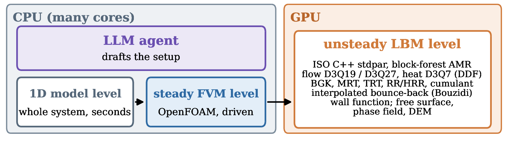
The LLM is a cloud LLM (Claude Code) today; it prepares code, scripts, cases and memory so that a local LLM can run the loop later (Architecture, Multi-fidelity).
The LBM kernel
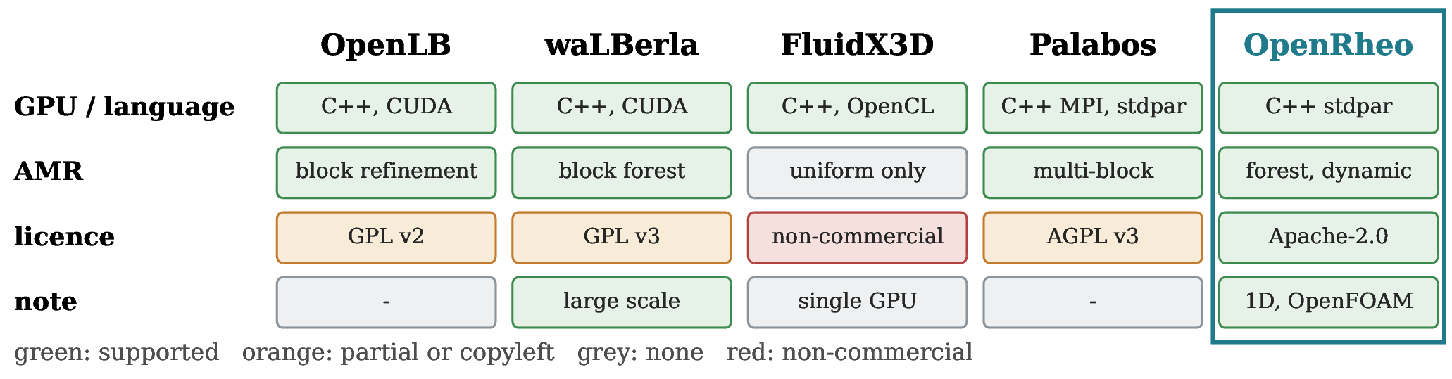
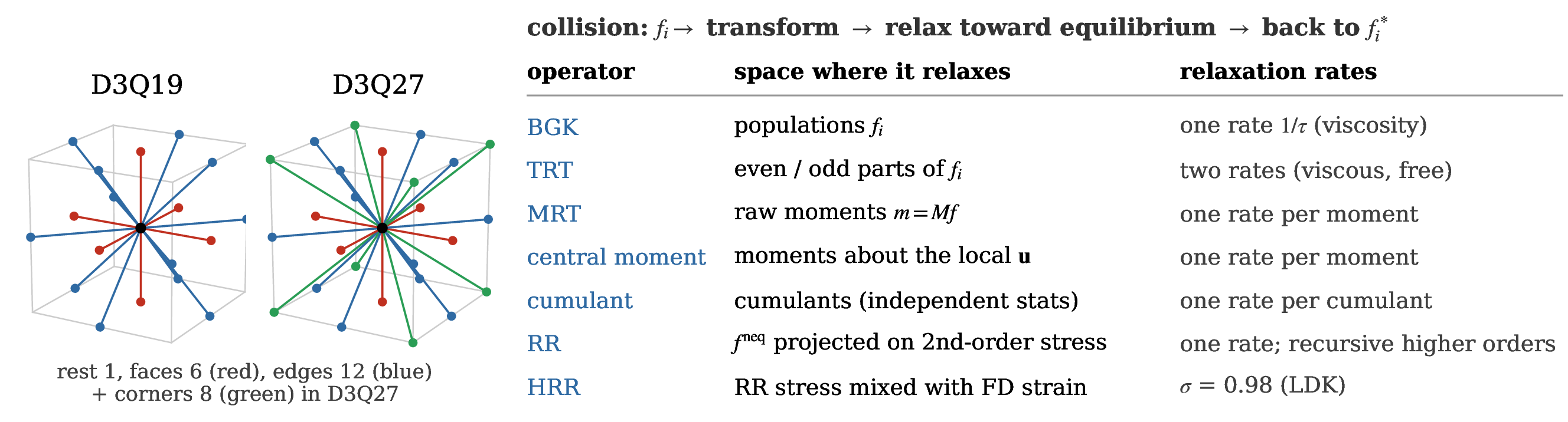
| Case | Animation | Against the reference |
|---|---|---|
| Cavity |  |
 |
| Ahmed body |  |
 |
| Dam break (SPHERIC) |  |
 |
| Natural convection |  |
 |
| Blood flow (aneurysm) |  |
 |
| Wind environment (AIJ case A) |  |
 |
| DEM (two spheres) |  |
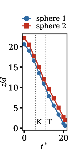 |
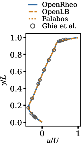
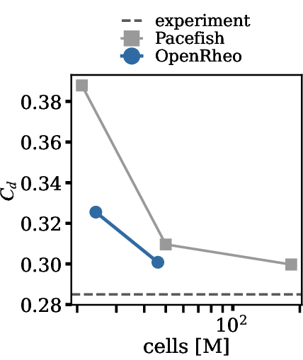
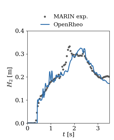
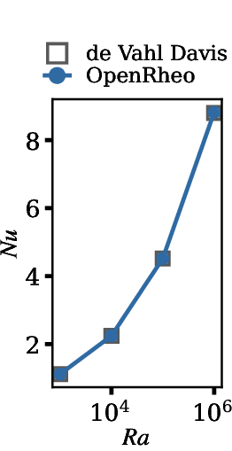
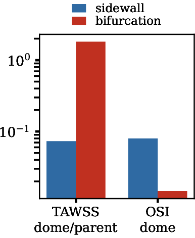
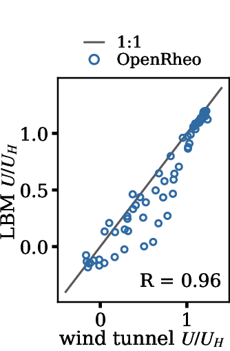
Blue is OpenRheo, grey the reference (experiment or analysis); most agree, the Ahmed body Cd is about 10 % high. The animations were re-run for visualisation.
ERCOFTAC case 41 (wall-mounted cube; D3Q27 cumulant LES, Smagorinsky Cs = 0.1, grid 1056 × 1152 × 96, Δx = H/48):
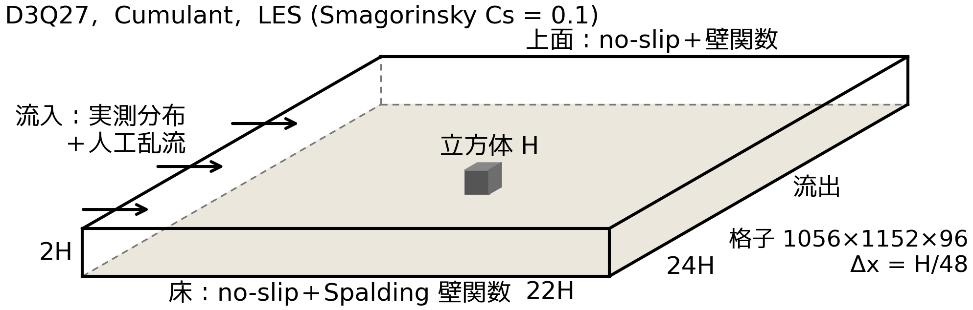
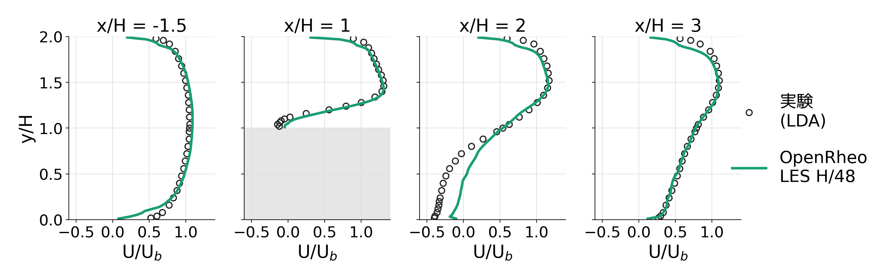
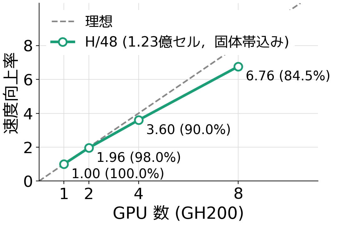
Details: Wall-mounted cube.
View factors by Monte Carlo
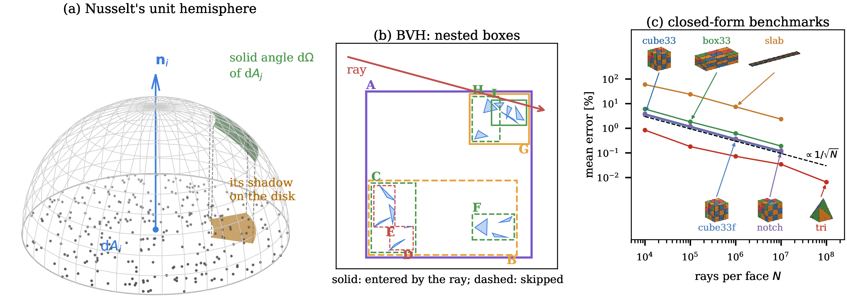
OpenFOAM's standard view factors are inaccurate and break the summation rule. Monte Carlo ray casting (cosine-weighted rays) satisfies the summation rule by construction; a BVH makes the ray tracing fast; symmetrising the product of area and view factor makes the reciprocity rule hold as well. Verified on shapes with closed-form solutions (viewFactorsGenMC, GPLv3).
Apartment LDK: steady FVM
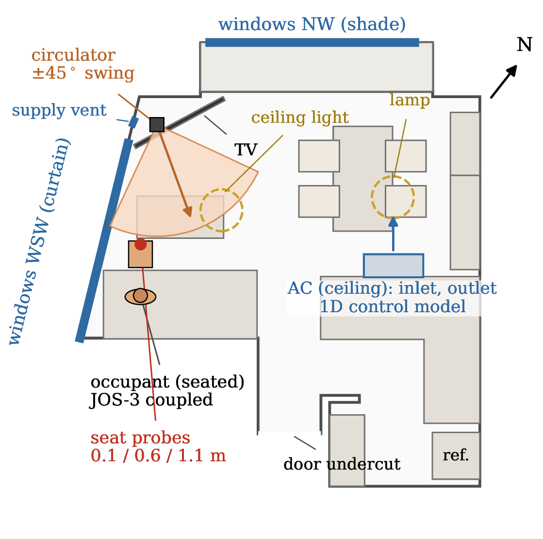
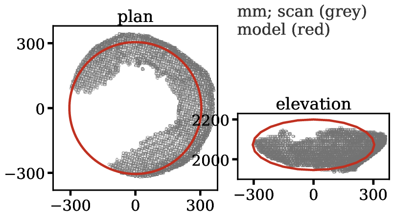
Mid-August, one adult seated on the sofa, air conditioner set to 27 °C. 53 surface temperatures (thermal camera) and 3 air temperatures (thermometer), 56 points in all; geometry from the floor and furniture plans and a smartphone LiDAR scan.
| Plan of the LDK | LiDAR scan (grey) and model (red) of a ceiling light |
|---|---|
 |
 |
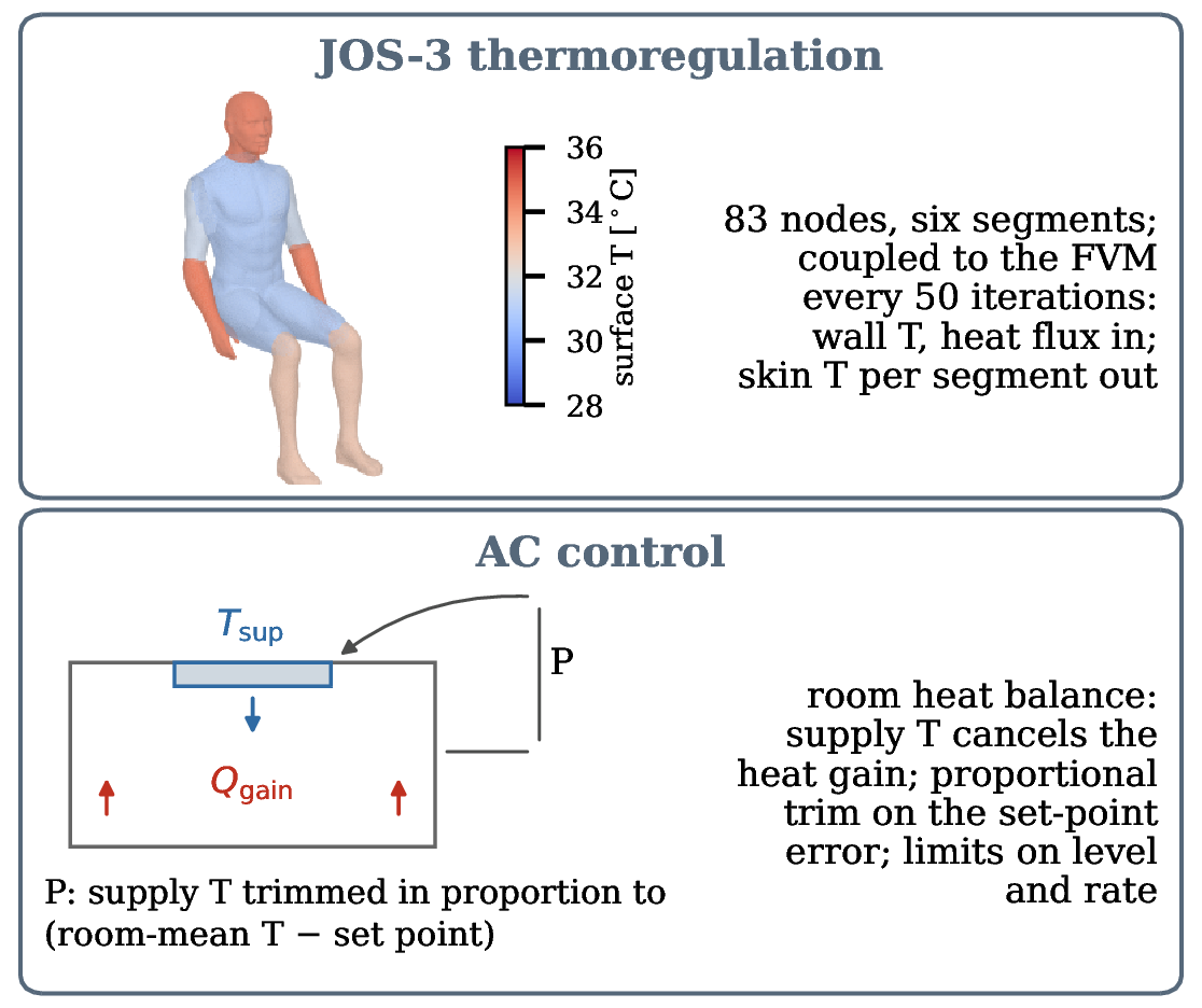
buoyantSimpleFoam with the radiation bug fixed, about 1.25 M cells (48 ranks), 30,000 iterations, k-ω SST, viewFactor with 4,440 coarse faces, the occupant coupled to JOS-3 (83 nodes) every 50 iterations, AC supply 0.196 kg/s at 22.0 °C (proportional control), heat gain 724 W / AC removal 946 W, outdoor 29.1 °C.
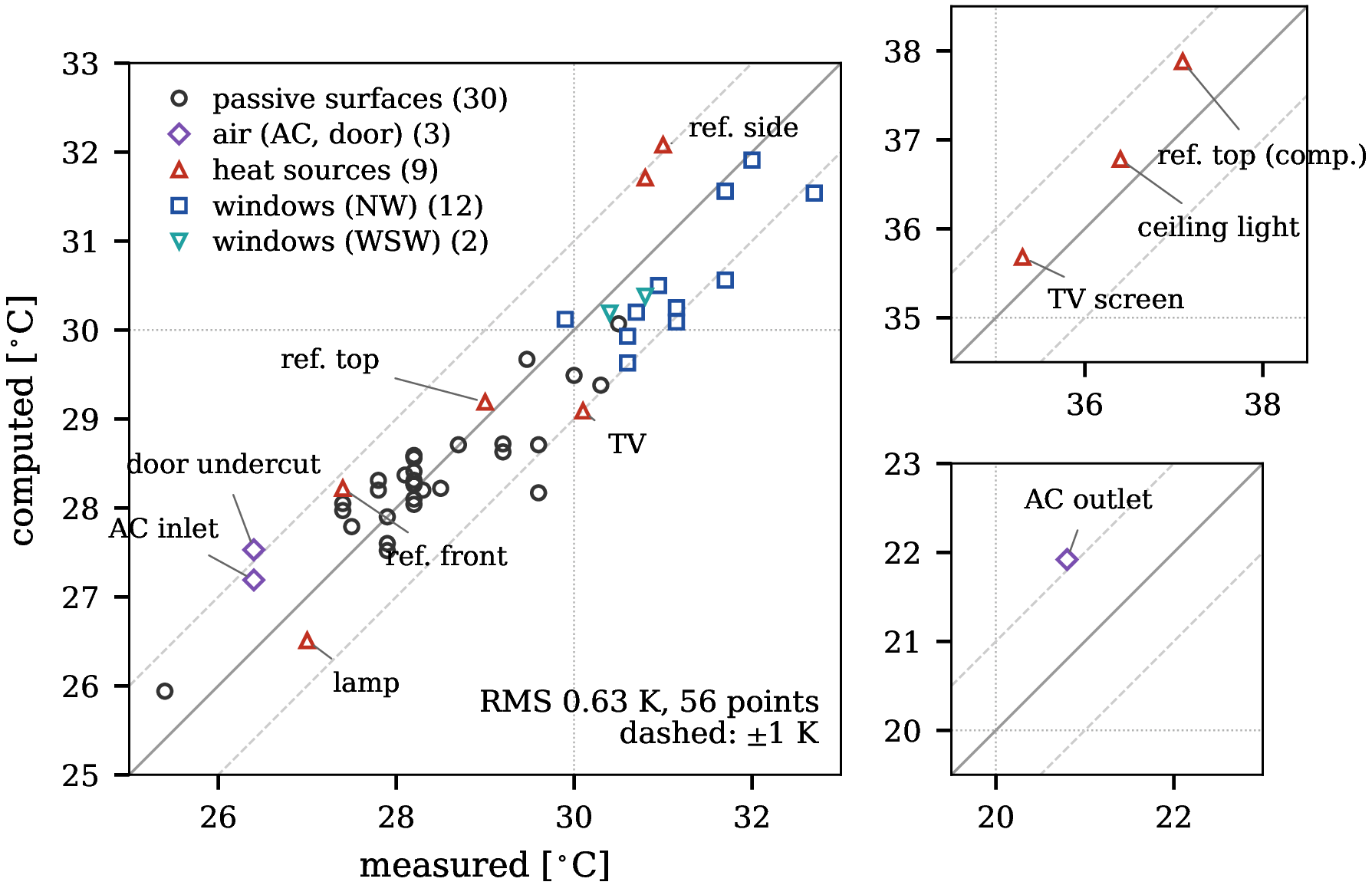
| Points | RMS [K] | Within ±1 K | |
|---|---|---|---|
| Not windows | 42 | 0.60 | 37 |
| Windows | 14 | 0.69 | 11 |
| All | 56 | 0.63 | 48 |
Apartment LDK: unsteady LBM
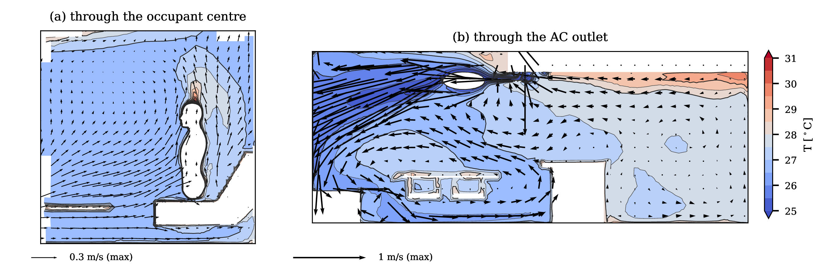
LBM alone missed the near-floor flow of the cold falling supply air (0.02 and 0.05 m/s at 0.1 and 0.6 m against the FVM's 0.25 and 0.21 m/s). So the steady FVM velocity and temperature are mapped onto the LBM grid as a base state held by a force and a heat source, and the LBM solves the fluctuation. Circulator off, and swinging (±45°, 60 s period) at 1/9, 2/9 and 4/9 flow, compared 30–90 s after the swing starts. D3Q19, 100 mm base refined in 3 levels to 12.5 mm (2.6 M fluid cells), HRR collision with Smagorinsky, Spalding wall function, Boussinesq.
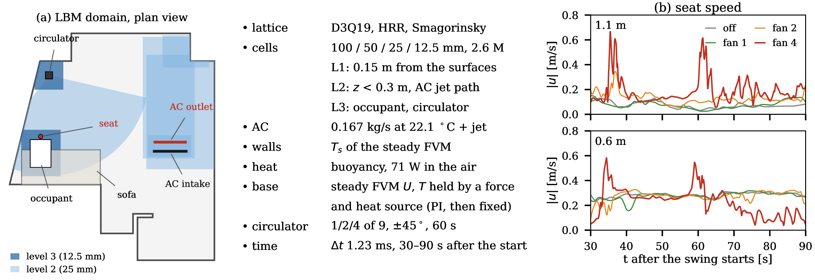
| (a) Horizontal section at the fan centre, 0.20 m | (b) Vertical section through the occupant (circulator elevation 18.5°) |
|---|---|
 |
 |
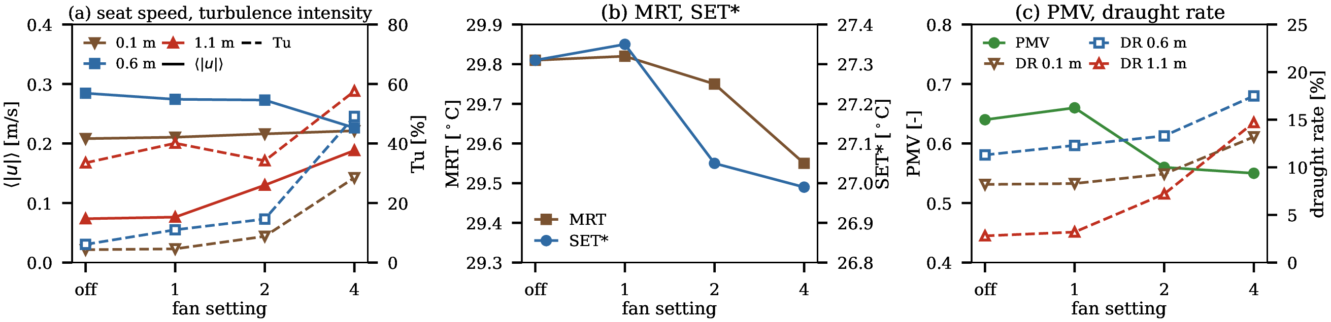
| At the seat | Off | Swing, flow 4/9 |
|---|---|---|
| Speed at the head (1.1 m) | 0.07 m/s | 0.19 m/s (+0.12 m/s) |
| Turbulence intensity Tu at the head | 34 % | 58 % (+24) |
| SET* | 27.3 °C | 27.0 °C (−0.3 °C, cooler) |
| PMV (0 neutral, positive warm) | 0.64 | 0.55 (−0.09, cooler) |
Car aerodynamics: DrivAer
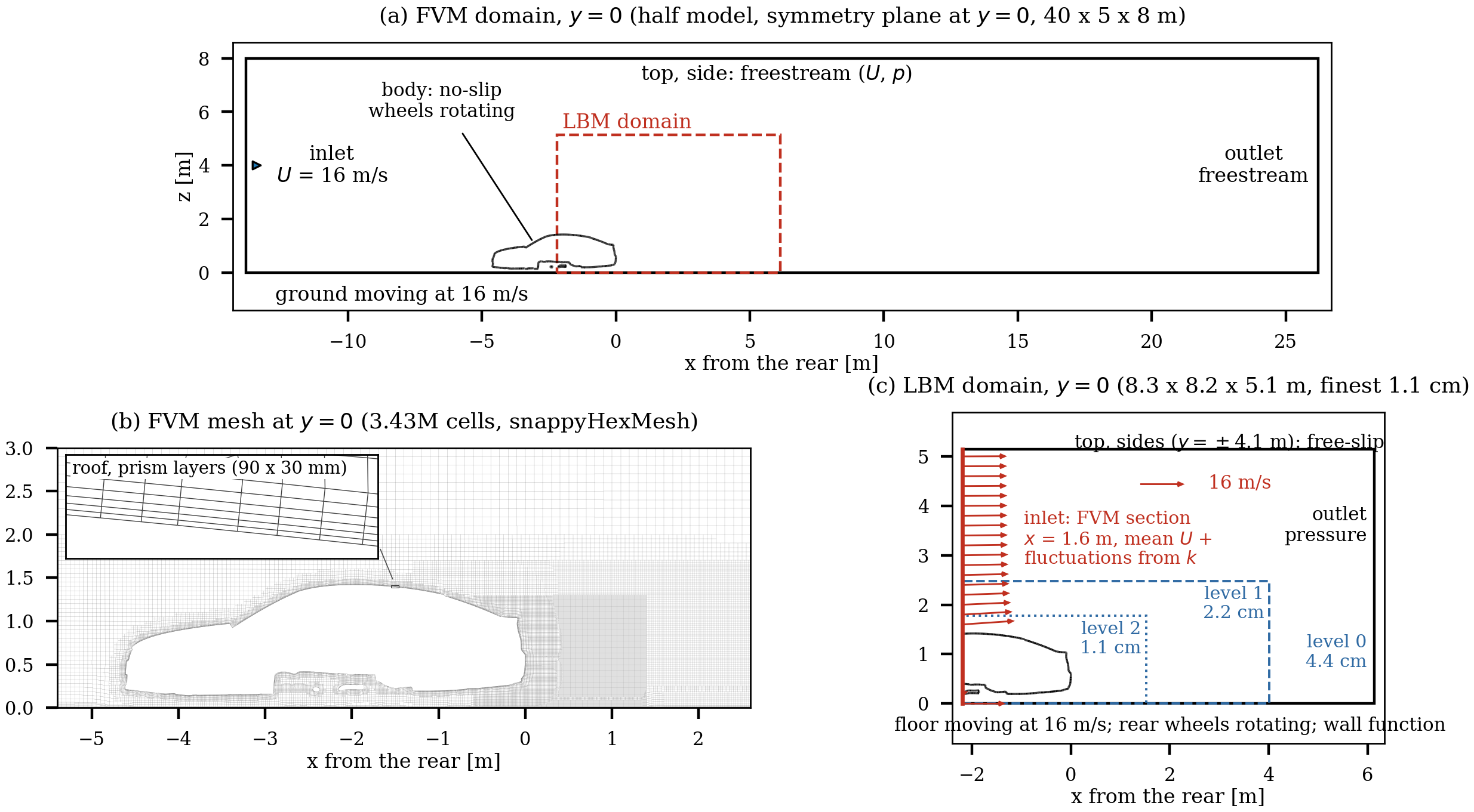
FVM: simpleFoam, k-ω SST, 3.43 M cells, rotating wheels, Cd 0.257 at 16 m/s (experiment [Collin] 0.252). LBM inflow: the FVM velocity plus digital-filter fluctuations from k. LBM: D3Q27 cumulant, finest 1.1 cm (19.82 M cells), about 45 minutes on one Miyabi-G GH200; Spalding wall function, moving floor, rotating rear wheels.
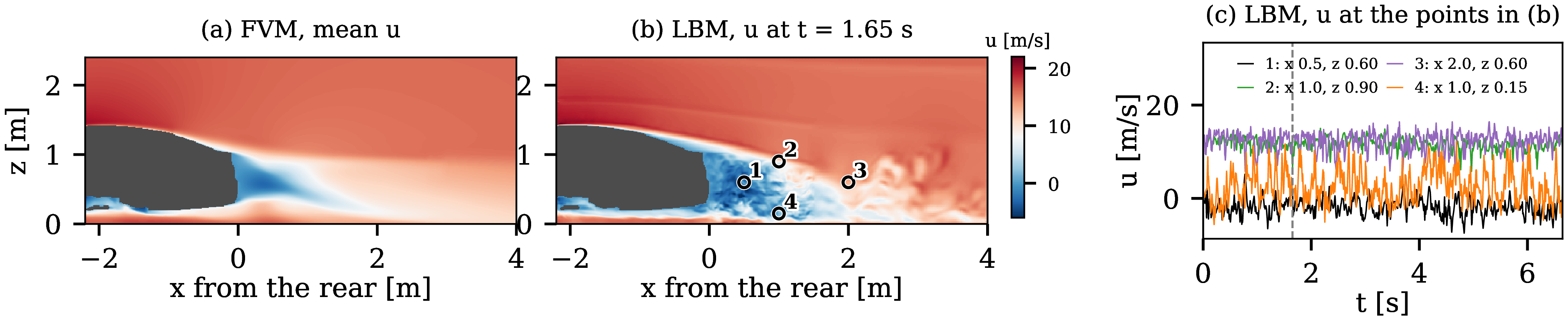
| FVM | LBM | LBM, underbody cells halved | |
|---|---|---|---|
| Rear recirculation length | 0.72 m | 0.92 m | 1.08 m |
| Speed 0.1 m above the floor at the rear | 12.8 m/s | 8.8 m/s | 12.6 m/s |
Wake standard deviation 1.2–3.4 m/s; spectral peaks 3.75–5.0 Hz (St = 0.33–0.44 on the car height). These are the abstract's runs; a rerun with the wall function relative to the moving floor and wheels gives 0.93 m and 9.4 m/s (Cd within 2 %).
Details: DrivAer fastback.
Mesh generation: rheoMesh
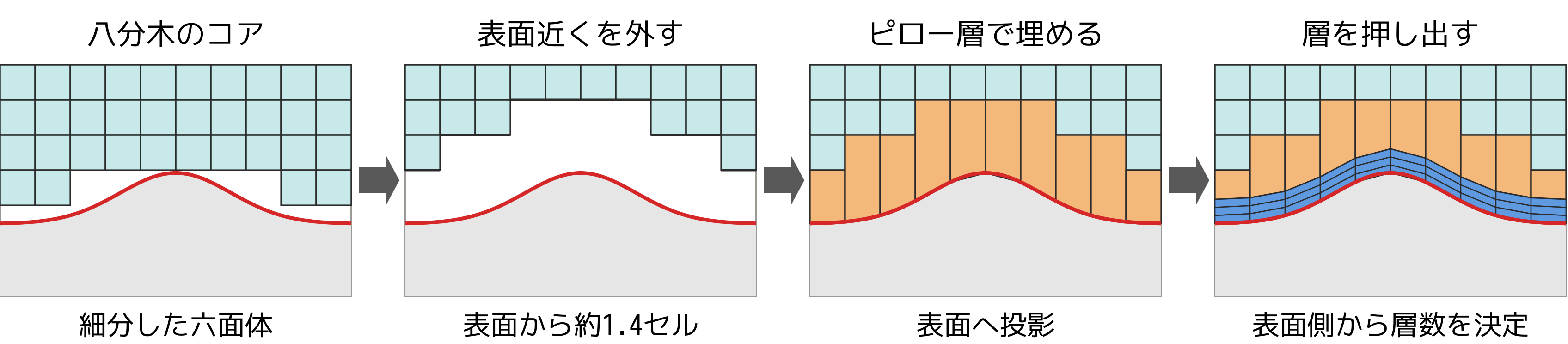
Written from scratch (the snappyHexMesh source was not read, for licence reasons); reads snappyHexMeshDict and the geometry as they are; the same octree gives the LBM block forest; no blockMesh and thread-parallel (oneTBB).
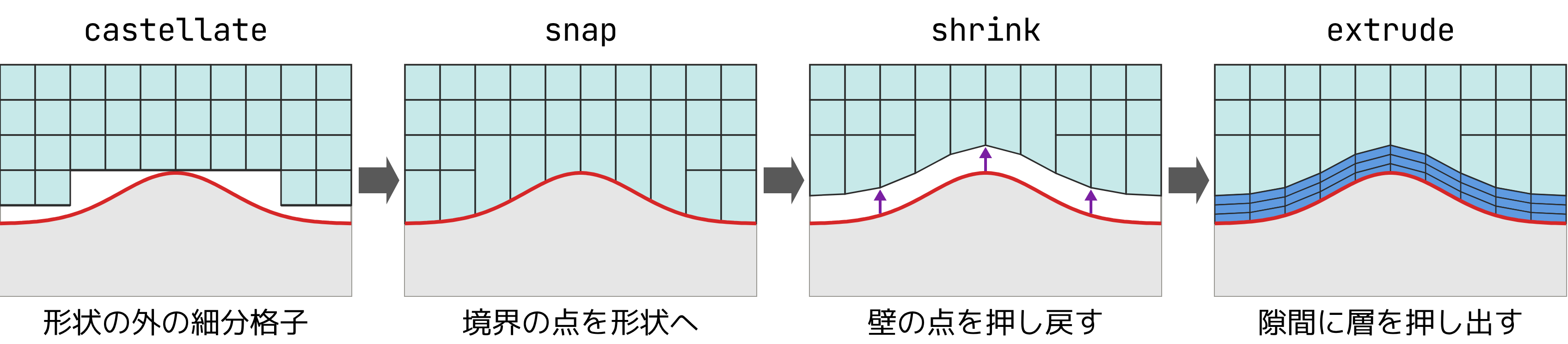
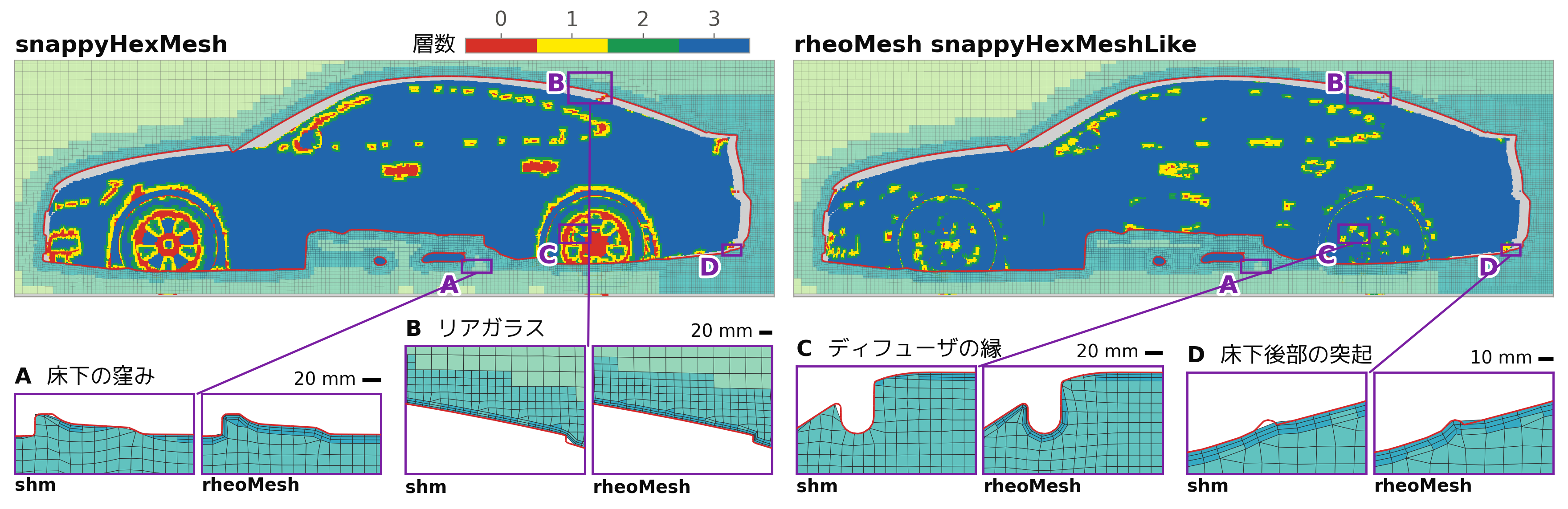
With the training-course settings (3 layers on body and wheels): mesher time 37.4 → 24.0 s with layers (30.7 → 8.2 s without), faces with non-orthogonality > 60° 52 → 39, skewness > 3 172 → 53, gap 841 → 149 cm³, layer coverage body 92.6 → 98.8 %, front wheels 58.1 → 94.0 %, rear wheels 54.9 → 94.4 % (Flow2 Type I, one node).

| 6 layers on body, wheels and ground | Cells | Time [s] | Non-orth > 60° | Feature edges ≤ 1 mm [%] | Gap [cm³] | Front-wheel coverage [%] | Front-wheel layers |
|---|---|---|---|---|---|---|---|
| shm | 3.43 M | 38.8 | 61 | 26.4 | 841 | 52.0 | 0.97 |
| rheoMesh (shm-like) | 3.54 M | 25.5 | 48 | 45.9 | 188 | 93.8 | 2.49 |
| rheoMesh (pillow) | 4.03 M | 60.4 (open) | 679 (open) | 57.1 | 121 | 96.4 | 5.51 |
Details: rheoMesh.
Summary and repositories
- OpenRheo, an AI-native multi-level analysis environment.
- View factors by Monte Carlo, symmetrised to meet both the summation and reciprocity rules.
- LDK steady FVM: RMS 0.60 K (not windows) and 0.69 K (windows) against measurement; windows biased by −0.55 K.
- LDK unsteady thermal LBM: the circulator swing raises turbulence intensity 34 → 58 % and lowers SET* 27.3 → 27.0 °C.
- Car aerodynamics: the wake solved by LBM with the steady FVM field as inflow gives unsteady results cheaply.
- rheoMesh: with the snappyHexMesh settings (3 layers on body and wheels) 37 s → 24 s, and missing wheel layers from over 40 % to under 10 %.
Next: control by a local LLM; the winter LDK (1D whole-house temperature and humidity, multi-objective optimisation of AC, floor heating and shades by steady FVM, draught by LBM — Pareto candidates from the CPU FVM checked by the GPU LBM).
- gitlab.com/masaz/openrheo: OpenRheo (LBM, test cases, 1D models such as the JOS-3 coupling, provisional rheoMesh)
- gitlab.com/masaz/viewFactorsGenMC: viewFactorsGenMC and the viewFactor bug-fix patch